What is Mathematics?
Mathematics
is the abstract study of topics such as quantity (numbers),[2] structure,[3] space,[2] and change.[4][5][6] There is a range of views among mathematicians and philosophers as to the exact scope and definition of mathematics.[7][8]
Mathematicians https://docs.google.com/forms/d/1XCKaP_E-F06OKzqqPcdTjdXhK1RTPxwznYK-J15ShtM/viewform. Mathematicians resolve the truth or falsity of conjectures by mathematical proof. When mathematical structures are good models of real phenomena, then mathematical reasoning can provide insight or predictions about nature. Through the use of abstraction and logic, mathematics developed from counting, calculation, measurement, and the systematic study of the shapes and motions of physical objects. Practical mathematics has been a human activity for as far back as written records exist. The research required to solve mathematical problems can take years or even centuries of sustained inquiry.
Rigorous arguments first appeared in Greek mathematics, most notably in Euclid's Elements. Since the pioneering work of Giuseppe Peano (1858–1932), David Hilbert (1862–1943), and others on axiomatic systems in the late 19th century, it has become customary to view mathematical research as establishing truth by rigorous deduction from appropriately chosen axioms and definitions. Mathematics developed at a relatively slow pace until the Renaissance, when mathematical innovations interacting with new scientific discoveries led to a rapid increase in the rate of mathematical discovery that has continued to the present day.[11]
Galileo Galilei (1564–1642) said, "The universe cannot be read until we have learned the language and become familiar with the characters in which it is written. It is written in mathematical language, and the letters are triangles, circles and other geometrical figures, without which means it is humanly impossible to comprehend a single word. Without these, one is wandering about in a dark labyrinth."[12] Carl Friedrich Gauss (1777–1855) referred to mathematics as "the Queen of the Sciences".[13] Benjamin Peirce (1809–1880) called mathematics "the science that draws necessary conclusions".[14] David Hilbert said of mathematics: "We are not speaking here of arbitrariness in any sense. Mathematics is not like a game whose tasks are determined by arbitrarily stipulated rules. Rather, it is a conceptual system possessing internal necessity that can only be so and by no means otherwise."[15] Albert Einstein (1879–1955) stated that "as far as the laws of mathematics refer to reality, they are not certain; and as far as they are certain, they do not refer to reality."[16] French mathematician Claire Voisin states "There is creative drive in mathematics, it's all about movement trying to express itself." [17]
Mathematics is used throughout the world as an essential tool in many fields, including natural science, engineering, medicine, finance and the social sciences. Applied mathematics, the branch of mathematics concerned with application of mathematical knowledge to other fields, inspires and makes use of new mathematical discoveries, which has led to the development of entirely new mathematical disciplines, such as statistics and game theory. Mathematicians also engage in pure mathematics, or mathematics for its own sake, without having any application in mind. There is no clear line separating pure and applied mathematics, and practical applications for what began as pure mathematics are often discovered.[18]
Etymology
The word mathematics comes from the Greek μάθημα (máthēma), which, in the ancient Greek language, means "that which is learnt",[24] "what one gets to know," hence also "study" and "science", and in modern Greek just "lesson." The word máthēma is derived from μανθάνω (manthano), while the modern Greek equivalent is μαθαίνω (mathaino), both of which mean "to learn." In Greece, the word for "mathematics" came to have the narrower and more technical meaning "mathematical study" even in Classical times.[25] Its adjective is μαθηματικός (mathēmatikós), meaning "related to learning" or "studious", which likewise further came to mean "mathematical". In particular, μαθηματικὴ τέχνη (mathēmatikḗ tékhnē), Latin: ars mathematica, meant "the mathematical art".
In Latin, and in English until around 1700, the term mathematics more commonly meant "astrology" (or sometimes "astronomy") rather than "mathematics"; the meaning gradually changed to its present one from about 1500 to 1800. This has resulted in several mistranslations: a particularly notorious one is Saint Augustine's warning that Christians should beware of mathematici meaning astrologers, which is sometimes mistranslated as a condemnation of mathematicians.
The apparent plural form in English, like the French plural form les mathématiques (and the less commonly used singular derivative la mathématique), goes back to the Latin neuter plural mathematica (Cicero), based on the Greek plural τα μαθηματικά (ta mathēmatiká), used by Aristotle (384–322 BC), and meaning roughly "all things mathematical"; although it is plausible that English borrowed only the adjective mathematic(al) and formed the noun mathematics anew, after the pattern of physics and metaphysics, which were inherited from the Greek.[26] In English, the noun mathematics takes singular verb forms. It is often shortened to maths or, in English-speaking North America, math.[27]
: Definitions of mathematics
Aristotle defined mathematics as "the science of quantity", and this definition prevailed until the 18th century.[28] Starting in the 19th century, when the study of mathematics increased in rigor and began to address abstract topics such as group theory and projective geometry, which have no clear-cut relation to quantity and measurement, mathematicians and philosophers began to propose a variety of new definitions.[29] Some of these definitions emphasize the deductive character of much of mathematics, some emphasize its abstractness, some emphasize certain topics within mathematics. Today, no consensus on the definition of mathematics prevails, even among professionals.[7] There is not even consensus on whether mathematics is an art or a science.[8] A great many professional mathematicians take no interest in a definition of mathematics, or consider it undefinable.[7] Some just say, "Mathematics is what mathematicians do."[7]
Three leading types of definition of mathematics are called logicist, intuitionist, and formalist, each reflecting a different philosophical school of thought.[30] All have severe problems, none has widespread acceptance, and no reconciliation seems possible.[30]
An early definition of mathematics in terms of logic was Benjamin Peirce's "the science that draws necessary conclusions" (1870).[31] In the Principia Mathematica, Bertrand Russell and Alfred North Whitehead advanced the philosophical program known as logicism, and attempted to prove that all mathematical concepts, statements, and principles can be defined and proven entirely in terms of symbolic logic. A logicist definition of mathematics is Russell's "All Mathematics is Symbolic Logic" (1903).[32]
Intuitionist definitions, developing from the philosophy of mathematician L.E.J. Brouwer, identify mathematics with certain mental phenomena. An example of an intuitionist definition is "Mathematics is the mental activity which consists in carrying out constructs one after the other."[30] A peculiarity of intuitionism is that it rejects some mathematical ideas considered valid according to other definitions. In particular, while other philosophies of mathematics allow objects that can be proven to exist even though they cannot be constructed, intuitionism allows only mathematical objects that one can actually construct.
Formalist definitions identify mathematics with its symbols and the rules for operating on them. Haskell Curry defined mathematics simply as "the science of formal systems".[33] A formal system is a set of symbols, or tokens, and some rules telling how the tokens may be combined into formulas. In formal systems, the word axiom has a special meaning, different from the ordinary meaning of "a self-evident truth". In formal systems, an axiom is a combination of tokens that is included in a given formal system without needing to be derived using the rules of the system.(http://en.wikipedia.org/wiki/Mathematics).
The
Divisions of Mathematics
In order to find one's way around the collection of mathematical ideas, it is useful to organize them and classify them in some way into parts.
Among the ways to divide the field of mathematics is by field of application. There are many books and courses in schools labeled "Engineering mathematics", "Financial mathematics", "Mathematics for social scientists", and so on. While it is perhaps easier for the reader to have the material pre-filtered according to application, this hides the fact that the underlying mathematics is really quite similar --- radioactive decay is essentially the same as inflationary depreciation of investments, for example. At this site we emphasize the mathematics itself rather than the intended application, so this method of dividing material is inappropriate for us.
Another way to divide the portions of mathematics is by level of complexity. Elementary topics include arithmetic and measurement; intermediate topics include simple algebra and plane geometry. From there we may pass to somewhat more complex topics built upon these: trigonometry, "advanced" algebra, analytic geometry, and calculus.
This website is limited to topics more advanced than these; little mention will be made of topics which are typically not considered (except in their most elementary aspects) until a student has progressed through some University studies. Our intended audience at the site is the person who has already studied some mathematics courses beyond these at the university level, although in this tour we try to be more inclusive.
That said, we proceed to divide mathematics along thematic lines.
How many parts of mathematics -- Two? Eight? Sixty-three?
[A map of the fields of mathematics]
The image at right shows a "map" of the subfields of mathematics. These are the major classification groupings used at this site and by most research mathematics projects. The sizes and positions of the "bubbles" are computed to reflect the sizes and relatedness of the various disciplines. On our tour, we'll highlight some of the main groupings of these areas (the different color groups).
One first step in dividing the mathematics literature is to decide which books and articles intend to reveal the structure of mathematics itself, and those which intend to apply mathematics to closely allied areas. This division between mathematics and its applications is of course vague. Indeed, we'll see that the two groups cut across each other on the MathMap.
The first group divides roughly into just a few broad overlapping areas:
Foundations considers questions in logic or set theory -- the very language of mathematics.
Algebra - is principally concerned with symmetry, patterns, discrete sets, and the rules for manipulating arithmetic operations; one might think of this as the outgrowth of arithmetic and algebra classes in primary and secondary school.
Geometry - is concerned with shapes and sets, and the properties of them which are preserved under various kinds of motions. Naturally this is related to elementary geometry and analytic geometry.
Analysis - studies functions, the real number line, and the ideas of continuity and limit; this is perhaps the natural successor to courses in graphing, trigonometry, and calculus. (This is a very large area; we subdivide it later into five areas which we may label Calculus and Real Analysis, Complex Analysis, Differential Equations, Theory of Functions, and Numerical Analysis and Optimization.)
Of course, the division of the subject areas into these broad headings is a little fuzzy: combinatorics is only weakly associated to the rest of "algebra"; Lie groups are arguably a part of analysis or topology instead of algebra, differential geometry is in practice closer to analysis than geometry, and so on.
The second broad part of the mathematics literature includes those areas which could be considered either independent disciplines or central parts of mathematics, as well as those areas which clearly use mathematics but involve non-mathematical ideas too. It is important to note that the collection of files at this site covers only the mathematical aspects of these subjects; we provide only cursory links to observational and experimental data, mathematically routine applications, computer paradigms, and so on.
Probability and Statistics, for example, has a dual nature -- mathematical and experimental. This classification scheme focuses on the former -- the study of the validity of the measurements one might make.
Computational sciences have obviously flourished in the last half-century, and consider algorithms and information handling. Here we are concerned with what might be computed, not with compilers, architectures, and so on.
Significant mathematics must be developed to formulate ideas in the physical sciences, engineering, and other branches of science. Again it is the theoretical underpinnings which concern us here rather than the experiment or tangible construction.
Finally note that every branch of mathematics has its own history, collections of important works -- reference, research, biographical, or expository -- and in many cases a suite of important algorithms. The MSC classification allows these topics to be included within each major heading at a secondary level. However, these themes are sometimes best woven together into areas of study which are not so much research into mathematics as research into the enterprise of mathematics -- "epi-mathematics", perhaps.
The Mathematics Subject Classification (MSC) scheme breaks down these general areas into 63 numbered subject classifications with widely varying characteristics. (This is the classification system used by the research mathematical societies.) We adhere to the polite fiction that these areas are more distinct than the subfields of some of the larger areas; more detail is available in the pages for the various areas.
Continue the tour by clicking on any of the major branches of mathematics described above. You might want to begin with a tour of foundations.
But is this division "real"?
In a word, "no". It's false to assume that mathematics consists of discrete subfields, it's false to assume that there is an objective way to gather those subfields into main divisions, and it's false to assume that there is an accurate two-dimensional positioning of the parts. For example, a division into "Pure" and "Applied" Mathematics is traditional, but the boundaries are unclear and cross-fertilization is common. Within the first part it is also traditional to identify Algebra, Geometry, and Analysis as the three largest areas, but again this division is somewhat artificial as we have noted.
Yet the picture we have described above is consistent with the images painted in other sources. Some other systems for classifying mathematics are presented for browsing in the set of subject headings used at this site. Each system is different and yet it is generally possible to match parts of one classification scheme with parts of another.
The National Science Foundation, for example, organizes its mathematics programs into
1.) Algebra and Number Theory
2.) Topology and Foundations
3.) Geometric Analysis
4.) Analysis
5.) Statistics and Probability
6.) Computational Mathematics
7.)Applied Mathematics
a division which clearly maintains the same larger areas we have indicated, though it gathers the smaller ones somewhat differently.
(http://www.math.niu.edu/~rusin/known-math/index/tour_div.html)
1.Foundation
The term foundations is used to refer to the formulation and analysis of the language, axioms, and logical methods on which all of mathematics rests (see logic; symbolic logic). The scope and complexity of modern mathematics requires a very fine analysis of the formal language in which meaningful mathematical statements may be formulated and perhaps be proved true or false. Most apparent mathematical contradictions have been shown to derive from an imprecise and inconsistent use of language. A basic task is to furnish a set of axioms effectively free of contradictions and at the same time rich enough to constitute a deductive source for all of modern mathematics. The modern axiom schemes proposed for this purpose are all couched within the theory of sets, originated by Georg Cantor, which now constitutes a universal mathematical language.
Read more: mathematics: Branches of Mathematics | Infoplease.com http://www.infoplease.com/encyclopedia/science/mathematics-branches-mathematics.html#ixzz2diYzBKrY
Read more: mathematics: Branches of Mathematics | Infoplease.com http://www.infoplease.com/encyclopedia/science/mathematics-branches-mathematics.html#ixzz2diYzBKrY
2.Algebra
Historically, algebra is the study of solutions of one or several algebraic equations, involving the polynomial functions of one or several variables. The case where all the polynomials have degree one (systems of linear equations) leads to linear algebra. The case of a single equation, in which one studies the roots of one polynomial, leads to field theory and to the so-called Galois theory. The general case of several equations of high degree leads to algebraic geometry, so named because the sets of solutions of such systems are often studied by geometric methods.
Modern algebraists have increasingly abstracted and axiomatized the structures and patterns of argument encountered not only in the theory of equations, but in mathematics generally. Examples of these structures include groups (first witnessed in relation to symmetry properties of the roots of a polynomial and now ubiquitous throughout mathematics), rings (of which the integers, or whole numbers, constitute a basic example), and fields (of which the rational, real, and complex numbers are examples). Some of the concepts of modern algebra have found their way into elementary mathematics education in the so-called new mathematics.
Some important abstractions recently introduced in algebra are the notions of category and functor, which grew out of so-called homological algebra. Arithmetic and number theory, which are concerned with special properties of the integers—e.g., unique factorization, primes, equations with integer coefficients (Diophantine equations), and congruences—are also a part of algebra. Analytic number theory, however, also applies the nonalgebraic methods of analysis to such problems.
Read more: mathematics: Branches of Mathematics | Infoplease.com http://www.infoplease.com/encyclopedia/science/mathematics-branches-mathematics.html#ixzz2diZ7u0Am
Algebra as a Branch of Mathematics
Algebra can essentially be considered as doing computations similar to that of
arithmetic with non-numerical mathematical
objects.[1] Initially, these objects represented either numbers that were not yet known (unknowns) or unspecified numbers (indeterminate or
parameter), allowing one to state and prove properties that are true no
matter which numbers are involved. For example, in the quadratic equation Ax^2 + Bx + C = 0 ; a,b,c are indeterminates and x is the unknown. Solving this equation amounts to computing with the variables
to express the unknowns in terms of the indeterminates. Then, substituting any
numbers for the indeterminates, gives the solution of a particular equation
after a simple arithmetic computation.
As it developed, algebra was extended to other non-numerical objects, like vectors, matrices or polynomials. Then, the structural properties of
these non-numerical objects were abstracted to define algebraic structures like groups, rings, fields and algebras.
Before the 16th century, mathematics was divided into only two subfields, arithmetic and geometry. Even though some methods, which had
been developed much earlier, may be considered nowadays as algebra, the
emergence of algebra and, soon thereafter, of infinitesimal
calculus as subfields of mathematics only dates from 16th or 17th
century. From the second half of 19th century on, many new fields of mathematics
appeared, some of them included in algebra, either totally or partially.
It follows that algebra, instead of being a true branch of mathematics,
appears nowadays, to be a collection of branches sharing common methods. This is
clearly seen in the Mathematics Subject Classification[2] where
none of the first level areas (two digit entries) is called algebra. In
fact, algebra is, roughly speaking, the union of sections 08-General algebraic
systems, 12-Field theory and polynomials, 13-Commutative algebra, 15-Linear and multilinear algebra; matrix theory, 16-Associative rings and algebras, 17-Nonassociative rings and algebras,
18-Category theory; homological algebra, 19-K-theory and 20-Group theory. Some other first level areas may be
considered to belong partially to algebra, like 11-Number theory (mainly for algebraic
number theory) and 14-Algebraic geometry.
Elementary Algebra
Elementary algebra encompasses some of the basic concepts of algebra, one of the main branches of mathematics. It is typically taught to secondary school students and builds on their
understanding of arithmetic. Whereas arithmetic deals with specified
numbers,[1] algebra
introduces quantities without fixed values, known as variables.[2] This use
of variables entails a use of algebraic notation and an understanding of the
general rules of the operators introduced in arithmetic. Unlike abstract algebra, elementary algebra is not concerned
with algebraic structures outside the realm of real and complex numbers.
The use of variables to denote quantities allows general relationships
between quantities to be formally and concisely expressed, and thus enables
solving a broader scope of problems. Most quantitative results in science and
mathematics are expressed as algebraic equations.
Algebraic notation
Algebraic notation describes how algebra is written. It follows certain rules
and conventions, and has its own terminology. For example, the expression 3x^2 - 2xy + C = 0
has the following components:
1 : Exponent (power), 2 : Coefficient, 3 : term, 4 : operator, 5 : constant,
: variables
A coefficient is a numerical value which multiplies a variable (the
operator is omitted). A term is an addend or a summand, a group of coefficients,
variables, constants and exponents that may be separated from the other terms by
the plus and minus operators.[3] Letters
represent variables and constants. By convention, letters at the beginning of
the alphabet ( a,b,c)are typically used to represent constants, and those toward the end of the
alphabet ( x, y and z )are used to represent variables.[4] They
are usually written in italics.[5]
.[5]
Algebraic operations work in the same way as arithmetic operations,[6] such
as addition, subtraction, multiplication, division
and exponentiation.[7] and
are applied to algebraic variables and terms. Multiplication symbols are usually
omitted, and implied when there is no space between two variables or terms, or
when a coefficient is used. For example 3 (x^2) is written as 3x^2 and 2(x)(y) can be writtten as 2xy.
Alternative notation
Other types of notation are used in algebraic expressions when the required
formatting is not available, or can not be implied, such as where only letters
and symbols are available. For example, exponents are usually formatted using
superscripts, e.g. . x^2
In plain text, and in the TeX mark-up language, the caret symbol "^" represents exponents, so
is written as "x^2".[12][13] In
programming languages such as Ada,[14] Fortran,[15] Perl,[16] Python [17] and
Ruby,[18] a
double asterisk is used, so x^2
is written as "x**2". Many programming languages and calculators use a single
asterisk to represent the multiplication symbol,[19] and
it must be explicitly used, for example, 3x
is written "3*x"..
Variables
Elementary algebra builds on and extends arithmetic[20] by introducing letters called variables to represent general (non-specified) numbers. This is useful for several reasons.
without
specifying the values of the quantities that are involved. For
example, it can be stated specifically that 5 minutes is equivalent to seconds. A more general (algebraic) description may state that the number of 60 x 5 = 300 seconds,
3.Variables allow one to describe mathematical relationships between
quantities that may vary.[23] For
example, the relationship between the circumference, c, and diameter,
d, of a circle is described by [ pie = c/d ].
4.Variables allow one to describe some mathematical properties.
For example, a basic property of addition is commutativity which states that the order of
numbers being added together does not matter. Commutativity is stated algebraically as . ( a+b ) = ( b+a ).
Abstract algebra
abstract algebra is a common name for the sub-area that studies
algebraic structures in their own right. Such
structures include groups, rings, fields, modules, vector spaces, and algebras. The specific term abstract
algebra was coined at the turn of the 20th century to distinguish this
area from the other parts of algebra. The term modern algebra
has also been used to denote abstract algebra.
Two mathematical subject areas that study the properties of algebraic
structures viewed as a whole are universal algebra and category
theory. Algebraic structures, together with the
associated homomorphisms, form categories. Category theory is a
powerful formalism for studying and comparing different algebraic
structures.
History
As in other parts of mathematics, concrete problems and examples have played
important roles in the development of algebra. Through the end of the nineteenth
century many, perhaps most of these problems were in some way related to the
theory of algebraic equations. Major themes include:
Numerous textbooks in abstract algebra start with axiomatic definitions of
various algebraic structures and then proceed to establish
their properties. This creates a false impression that in algebra axioms had
come first and then served as a motivation and as a basis of further study. The
true order of historical development was almost exactly the opposite. For
example, the hypercomplex numbers of the nineteenth century had
kinematic and physical motivations but challenged comprehension. Most theories
that are now recognized as parts of algebra started as collections of disparate
facts from various branches of mathematics, acquired a common theme that served
as a core around which various results were grouped, and finally became unified
on a basis of a common set of concepts. An archetypical example of this
progressive synthesis can be seen in the history
of group theory.
Early group
theory[edit source |
editbeta]
There were several threads in the early development of group theory, in
modern language loosely corresponding to number theory, theory of
equations, and geometry.
Leonhard Euler considered algebraic operations on numbers modulo an integer, modular arithmetic, in his
generalization of Fermat's little theorem. These investigations were
taken much further by Carl Friedrich Gauss, who considered the structure of
multiplicative groups of residues mod n and established many properties of cyclic and more general abelian groups that arise in this way. In his
investigations of composition of binary quadratic forms, Gauss
explicitly stated the associative law for the composition of forms, but
like Euler before him, he seems to have been more interested in concrete results
than in general theory. In 1870, Leopold Kronecker gave a definition of an abelian
group in the context of ideal class groups of a number field, generalizing
Gauss's work; but it appears he did not tie his definition with previous work on
groups, particularly permutation groups. In 1882, considering the same question,
Heinrich M. Weber realized the connection and gave a
similar definition that involved the cancellation property but omitted the existence of
the inverse element, which was sufficient in his context
(finite groups).
Permutations were studied by Joseph-Louis Lagrange in his 1770 paper Réflexions
sur la résolution algébrique des équations (Thoughts on Solving Algebraic
Equations) devoted to solutions of algebraic equations, in which he
introduced Lagrange resolvents. Lagrange's goal was to
understand why equations of third and fourth degree admit formulae for
solutions, and he identified as key objects permutations of the roots. An
important novel step taken by Lagrange in this paper was the abstract view of
the roots, i.e. as symbols and not as numbers. However, he did not consider
composition of permutations. Serendipitously, the first edition of Edward
Waring's Meditationes Algebraicae (Meditations on
Algebra) appeared in the same year, with an expanded version published in
1782. Waring proved the main theorem on symmetric functions, and specially
considered the relation between the roots of a quartic equation and its
resolvent cubic. Mémoire sur la résolution des équations (Memoire on
the Solving of Equations) of Alexandre Vandermonde (1771) developed the theory of
symmetric functions from a slightly different angle, but like Lagrange, with the
goal of understanding solvability of algebraic equations.
Kronecker claimed in 1888 that the study of modern algebra began with
this first paper of Vandermonde. Cauchy states quite clearly that Vandermonde
had priority over Lagrange for this remarkable idea, which eventually led to the
study of group theory.[1]
Paolo
Ruffini was the first person to develop the theory of permutation groups, and like his predecessors, also
in the context of solving algebraic equations. His goal was to establish the
impossibility of an algebraic solution to a general algebraic equation of degree
greater than four. En route to this goal he introduced the notion of the order
of an element of a group, conjugacy, the cycle decomposition of elements of
permutation groups and the notions of primitive and imprimitive and proved some
important theorems relating these concepts, such as
if G is a subgroup of S5 whose order is
divisible by 5 then G contains an element of order 5.
Note, however, that he got by without formalizing the concept of a group, or
even of a permutation group. The next step was taken by Évariste Galois in 1832, although his work remained
unpublished until 1846, when he considered for the first time what is now called
the closure property of a group of permutations, which he expressed
as
... if in such a group one has the substitutions S and T then one has the
substitution ST.
The theory of permutation groups received further far-reaching development in
the hands of Augustin Cauchy and Camille Jordan, both through introduction of new
concepts and, primarily, a great wealth of results about special classes of
permutation groups and even some general theorems. Among other things, Jordan
defined a notion of isomorphism, still in the context of permutation
groups and, incidentally, it was he who put the term group in wide
use.
The abstract notion of a group appeared for the first time in Arthur
Cayley's papers in 1854. Cayley realized that a group need not be a
permutation group (or even finite), and may instead consist of matrices, whose algebraic properties, such as
multiplication and inverses, he systematically investigated in succeeding years.
Much later Cayley would revisit the question whether abstract groups were more
general than permutation groups, and establish that, in fact, any group is
isomorphic to a group of permutations.
Modern algebra
The end of the 19th and the beginning of the 20th century saw a tremendous
shift in the methodology of mathematics. Abstract algebra emerged around the
start of the 20th century, under the name modern algebra. Its study was
part of the drive for more intellectual rigor in mathematics. Initially, the
assumptions in classical algebra, on which the whole of mathematics (and major
parts of the natural sciences) depend, took the form of axiomatic systems. No longer satisfied with
establishing properties of concrete objects, mathematicians started to turn
their attention to general theory. Formal definitions of certain algebraic structures began to emerge in the 19th
century. For example, results about various groups of permutations came to be
seen as instances of general theorems that concern a general notion of an
abstract group. Questions of structure and classification of various
mathematical objects came to forefront.
These processes were occurring throughout all of mathematics, but became
especially pronounced in algebra. Formal definition through primitive operations
and axioms were proposed for many basic algebraic structures, such as groups, rings, and fields. Hence such things as group
theory and ring theory took their places in pure
mathematics. The algebraic investigations of general fields by Ernst Steinitz and of commutative and then general
rings by David Hilbert, Emil Artin and Emmy Noether, building up on the work of Ernst
Kummer, Leopold Kronecker and Richard Dedekind, who had considered ideals in
commutative rings, and of Georg Frobenius and Issai Schur, concerning representation theory of
groups, came to define abstract algebra. These developments of the last quarter
of the 19th century and the first quarter of 20th century were systematically
exposed in Bartel van der Waerden's Moderne algebra, the
two-volume monograph published in 1930–1931 that forever changed
for the mathematical world the meaning of the word algebra from the
theory of equations to the theory of algebraic structures.
Basic concepts[edit source |
editbeta]
Main article: Algebraic structures
By abstracting away various amounts of detail, mathematicians have created
theories of various algebraic structures that apply to many objects. For
instance, almost all systems studied are sets, to which the theorems of set
theory apply. Those sets that have a certain binary operation defined
on them form magmas, to which the concepts concerning magmas, as
well those concerning sets, apply. We can add additional constraints on the
algebraic structure, such as associativity (to form semigroups);
associativity, identity, and inverses (to form groups); and other more complex structures. With
additional structure, more theorems could be proved, but the generality is
reduced. The "hierarchy" of algebraic objects (in terms of generality) creates a
hierarchy of the corresponding theories: for instance, the theorems of group
theory apply to rings (algebraic objects that have two binary
operations with certain axioms) since a ring is a group over one of its
operations. Mathematicians choose a balance between the amount of generality and
the richness of the theory.
Linear Algebra
Linear algebra is the branch of mathematics concerning vector spaces, often finite or countably infinite dimensional, as well as linear
mappings between such spaces. Such an investigation is initially
motivated by a system of linear equations containing several
unknowns. Such equations are naturally represented using the formalism of matrices and vectors.[1]
Linear algebra is central to both pure and applied mathematics. For instance,
abstract algebra arises by relaxing the axioms of a
vector space, leading to a number of generalizations. Functional analysis studies the infinite-dimensional
version of the theory of vector spaces. Combined with calculus, linear algebra
facilitates the solution of linear systems of differential equations. Techniques from linear
algebra are also used in analytic geometry, engineering, physics, natural sciences, computer science, computer animation, and the social
sciences (particularly in economics). Because linear algebra is such a
well-developed theory, nonlinear mathematical models are sometimes approximated by
linear ones.
History
The study of linear algebra first emerged from the study of determinants, which were used to solve systems of
linear equations. Determinants were used by Leibniz
in 1693, and subsequently, Gabriel Cramer devised Cramer's Rule for solving linear systems in 1750.
Later, Gauss further developed the theory of solving linear
systems by using Gaussian elimination, which was initially listed as
an advancement in geodesy.[2]
The study of matrix algebra first emerged in England in the mid-1800s. In
1844 Hermann Grassmann published his “Theory of Extension”
which included foundational new topics of what is today called linear algebra.
In 1848, James Joseph Sylvester introduced the term matrix,
which is Latin for "womb". While studying compositions of linear
transformations, Arthur Cayley was led to define matrix multiplication
and inverses. Crucially, Cayley used a single letter to denote a matrix, thus
treating a matrix as an aggregate object. He also realized the connection
between matrices and determinants, and wrote "There would be many things to say
about this theory of matrices which should, it seems to me, precede the theory
of determinants".[3]
In 1882, Hüseyin Tevfik Pasha wrote the book titled "Linear
Algebra".[4][5] The first
modern and more precise definition of a vector space was introduced by Peano in 1888;[3] by 1900, a
theory of linear transformations of finite-dimensional vector spaces had
emerged. Linear algebra first took its modern form in the first half of the
twentieth century, when many ideas and methods of previous centuries were
generalized as abstract algebra. The use of matrices in quantum mechanics, special relativity, and statistics helped spread the subject of linear
algebra beyond pure mathematics. The development of computers led to increased
research in efficient algorithms for Gaussian elimination and matrix
decompositions, and linear algebra became an essential tool for modelling and
simulations.[3]
The origin of many of these ideas is discussed in the articles on determinants and Gaussian elimination.
Gaussian elimination
In linear algebra, Gaussian elimination (also
known as row reduction) is an algorithm for solving systems
of linear equations. It is usually understood as a sequence of
operations performed on the associated matrix of coefficients. This method can also be used
to find the rank of a matrix, to calculate the determinant of a matrix, and to calculate the inverse
of an invertible square matrix. The method is named after
Carl Friedrich Gauss, although it was known to
Chinese mathematicians as early as 179 CE (see History section).
To perform row reduction on a matrix, one uses a sequence of elementary row operations to modify the matrix until
the lower left-hand corner of the matrix is filled with zeros, as much as is
possible. There are three types of elementary row operations: 1) Swapping two
rows, 2) Multiplying a row by a non-zero number, 3) Adding a multiple of one row
to another row. Using these operations a matrix can always be transformed into
an upper triangular matrix, and in fact one that is in
row
echelon form. Once all of the leading coefficients (the left-most
non-zero entry in each row) are 1, and in every column containing a leading
coefficient has zeros elsewhere, the matrix is said to be in reduced row echelon form. This final form is unique;
in other words, it is independent of the sequence of row operations used. For
example, in the following sequence of row operations (where multiple elementary
operations might be done at each step), the third and fourth matrices are the
ones in row echelon form, and the final matrix is the unique reduced row echelon
form.In linear algebra, Gaussian elimination (also
known as row reduction) is an algorithm for solving systems
of linear equations. It is usually understood as a sequence of
operations performed on the associated matrix of coefficients. This method can also be used
to find the rank of a matrix, to calculate the determinant of a matrix, and to calculate the inverse
of an invertible square matrix. The method is named after
Carl Friedrich Gauss, although it was known to
Chinese mathematicians as early as 179 CE (see History section).
To perform row reduction on a matrix, one uses a sequence of elementary row operations to modify the matrix until
the lower left-hand corner of the matrix is filled with zeros, as much as is
possible. There are three types of elementary row operations: 1) Swapping two
rows, 2) Multiplying a row by a non-zero number, 3) Adding a multiple of one row
to another row. Using these operations a matrix can always be transformed into
an upper triangular matrix, and in fact one that is in
row
echelon form. Once all of the leading coefficients (the left-most
non-zero entry in each row) are 1, and in every column containing a leading
coefficient has zeros elsewhere, the matrix is said to be in reduced row echelon form. This final form is unique;
in other words, it is independent of the sequence of row operations used. For
example, in the following sequence of row operations (where multiple elementary
operations might be done at each step), the third and fourth matrices are the
ones in row echelon form, and the final matrix is the unique reduced row echelon
form.
Vector spaces[edit source |
editbeta]
The main structures of linear algebra are vector spaces. A vector space over a field F is a set V together with two binary operations. Elements of V are called
vectors and elements of F are called scalars. The
first operation, vector addition, takes any two vectors v
and w and outputs a third vector v +
w. The second operation takes any scalar a and any vector
v and outputs a new vector vector av.
In view of the first example, where the multiplication is done by rescaling the
vector v by a scalar a, the multiplication is called scalar multiplication of v by a.
The operations of addition and multiplication in a vector space satisfy the
following axioms.[6] In the
list below, let u, v and w be arbitrary vectors in
V, and a and b scalars in F.
Axiom
Signification
Associativity
of addition
u + (v + w) = (u + v) +
w
Commutativity
of addition
u + v = v + u
Identity
element of addition
There exists an element 0 ∈ V, called the zero
vector, such that v + 0 = v for all v ∈
V.
Inverse
elements of addition
For every v ∈ V, there exists an element −v ∈ V, called
the additive
inverse of v, such that v + (−v) = 0
Distributivity
of scalar multiplication with respect to vector addition
a(u + v) = au + av
Distributivity of scalar multiplication with respect to field addition
(a + b)v = av + bv
Compatibility of scalar multiplication with field multiplication
a(bv) = (ab)v [nb
1]
Identity element of scalar multiplication
1v = v, where 1 denotes the multiplicative
identity in F.
Elements of a general vector space V may be objects of any nature, for
example, functions, polynomials, vectors, or matrices. Linear algebra is
concerned with properties common to all vector spaces.
Linear
transformations[edit source |
editbeta]
Similarly as in the theory of other algebraic structures, linear algebra
studies mappings between vector spaces that preserve the vector-space structure.
Given two vector spaces V and W over a field F, a linear transformation (also called linear map, linear
mapping or linear operator) is a map
Commutative algebra
Commutative algebra is the branch of abstract algebra that studies commutative rings, their ideals, and modules over such rings. Both algebraic geometry and algebraic number theory build on commutative algebra. Prominent examples of
commutative rings include polynomial rings, rings of algebraic integers, including the ordinary integers ,
and p-adic integers z. Commutative algebra is the main technical tool in the local study of schemes.
The study of rings which are not necessarily commutative is known as noncommutative algebra; it includes ring
theory, representation theory, and the theory of Banach
algebras.
History
The subject, first known as ideal theory, began with Richard Dedekind's work on ideals, itself based on the earlier work of Ernst Kummer and Leopold Kronecker. Later, David
Hilbert introduced the term ring to generalize the earlier
term number ring. Hilbert introduced a more abstract approach to replace
the more concrete and computationally oriented methods grounded in such things
as complex analysis and classical invariant theory. In turn, Hilbert strongly
influenced Emmy Noether, who recast many earlier results in
terms of an ascending chain condition, now known as the
Noetherian condition. Another important milestone was the work of Hilbert's
student Emanuel Lasker, who introduced primary ideals and proved the first version of
the Lasker–Noether theorem.
The main figure responsible for the birth of commutative algebra as a mature
subject was Wolfgang Krull, who introduced the fundamental
notions of localization and completion
of a ring, as well as that of regular local rings. He established the concept
of the Krull dimension of a ring, first for Noetherian rings before moving on to expand his
theory to cover general valuation rings and Krull rings. To this day, Krull's principal ideal theorem is widely
considered the single most important foundational theorem in commutative
algebra. These results paved the way for the introduction of commutative algebra
into algebraic geometry, an idea which would revolutionize the latter
subject.
Much of the modern development of commutative algebra emphasizes modules.
Both ideals of a ring R and R-algebras are special cases of
R-modules, so module theory encompasses both ideal theory and the theory
of ring extensions. Though it was already incipient
in Kronecker's work, the modern approach to
commutative algebra using module theory is usually credited to Krull and Noether.
computer algebra / Symbolic computation
computer algebra, also called symbolic computation or
algebraic computation is a scientific area that refers to the study and
development of algorithms and software for manipulating mathematical
expressions and other mathematical objects. Although, properly speaking,
computer algebra should be a subfield of scientific computing, they are generally considered
as a distinct field because scientific computing is usually based on numerical computation with approximate floating point numbers, while computer algebra
emphasizes exact computation with expressions containing variables that have not any given value and are thus
manipulated as symbols (therefore the name of symbolic computation).
Software
applications that perform symbolic calculations are called computer
algebra systems, with the term system alluding to the
complexity of the main applications that include, at least, a method to
represent mathematical data in a computer, a user programming language (usually
different from the language used for the implementation), a dedicated memory
manager, a user interface for the input/output of mathematical
expressions, a large set of routines
to perform usual operations, like simplification of expressions, differentiation using chain rule, polynomial
factorization, indefinite integration, etc.
At the beginning of computer algebra, circa 1970, when the long-known algorithms
were first put on computers, they turned out to be highly inefficient.[1] Therefore,
a large part of the work of the searchers in the field consisted in revisiting
classical algebra in order to make it effective and to discover efficient algorithms to implement this effectiveness.
A typical example of this kind of work is the computation of polynomial greatest common divisors, which is
required to simplify fractions. Almost everything in that article, that is
behind the classical Euclid's algorithm, has been introduced for the need of
computer algebra.
Computer algebra is widely used to experiment in mathematics and to design
the formulas that are used in numerical programs. It is also used for complete
scientific computations, when purely numerical methods fail, like in public key cryptography or for some non-linear
problems.
Terminology
Some authors distinguish computer algebra from symbolic
computation using the latter name to refer to kinds of symbolic computation
other than the computation with mathematical formulas. Some authors use
symbolic computation for the computer science aspect of the subject and
"computer algebra" for the mathematical aspect.[2] In some
languages the name of the field is not a direct translation of its English name.
Typically, it is called calcul formel in French, which means "formal
computation".
Symbolic computation has also been referred to, in the past, as symbolic
manipulation, algebraic manipulation, symbolic processing,
symbolic mathematics, or symbolic algebra, but these terms, which
also refer to non-computational manipulation, are no more in use for referring
to computer algebra.
Data
representation[edit source |
editbeta]
As numerical software are highly efficient for
approximate numerical computation, it is common, in computer
algebra, to emphasize on exact computation with exactly represented data.
Such an exact representation implies that, even when the size of the output is
small, then the intermediate data that are generated during a computation may
grow in an unpredictable way. This behavior is called expression swell.
To obviate to this problem, various methods are used in the representation of
the data, as well as in the algorithms that manipulate them.
Numbers
The usual numbers systems used in numerical computation are either the floating point numbers and the integers
of a fixed bounded size, that are improperly called integers by most programming languages. None is convenient for
computer algebra, because of the expression swell.
Therefore, the basic numbers used in computer algebra are the integers of the
mathematicians, commonly represented by a unbounded signed sequence of digits in some base of numeration, usually the largest base allowed
by the machine word. These integers allow to define the rational numbers, which are irreducible fractions of two integers.
Programming an efficient implementation of the arithmetic operations is a
hard task. Therefore, most free computer algebra systems and some commercial ones,
like Maple (software), use the GMP library, which is thus a de facto
standard.
Expressions
Except for numbers and variables, every mathematical
expression may be viewed as the symbol of an operator followed by a
sequence
of operands. In computer algebra software, the expressions are usually
represented in this way. This representation is very flexible, and many things,
that seem not to be mathematical expressions at first glance, may be represented
and manipulated as such. For example, an equation is an expression with “=” as
an operator, a matrix may be represented as an expression with “matrix” as an
operator and its rows as operands.
Even programs may be considered and represented as expressions with operator
“procedure” and, at least, two operands, the list of parameters and the body,
which is itself an expression with “body” as an operator and a sequence of
instructions as operands. Conversely, any mathematical expression may be viewed
as a program. For example, the expression a
+ b may be viewed as a program for the addition, with a and b as parameters. Executing this program consists
in evaluating the expression for given values of a and b; if they do not have
any value—that is they are indeterminates—, the result of the evaluation is
simply its input.
This process of delayed evaluation is fundamental in computer algebra. For
example, the operator “=” of the equations is also, in most computer algebra
systems, the name of the program of the equality test: normally, the evaluation
of an equation results in an equation, but, when an equality test is
needed,—either explicitly asked by the user through an “evaluation to a Boolean”
command, or automatically started by the system in the case of a test inside a
program—then the evaluation to a boolean 0 or 1 is executed.
As the size of the operands of an expression is unpredictable and may change
during a working session, the sequence of the operands is usually represented as
a sequence of either pointers (like in Macsyma) or entries in a hash table (like in Maple).
Homological algebra
Homological algebra is the branch of mathematics that studies homology in a general algebraic setting. It is a relatively young discipline, whose origins can be traced to investigations in combinatorial topology (a precursor to algebraic topology) and abstract algebra (theory of modules and syzygies) at the end of the 19th century, chiefly by Henri Poincaré and David Hilbert.
The development of homological algebra was closely intertwined with the emergence of category theory. By and large, homological algebra is the study of homological functors and the intricate algebraic structures that they entail. One quite useful and ubiquitous concept in mathematics is that of chain complexes, which can be studied both through their homology and cohomology. Homological algebra affords the means to extract information contained in these complexes and present it in the form of homological invariants of rings, modules, topological spaces, and other 'tangible' mathematical objects. A powerful tool for doing this is provided by spectral sequences.
From its very origins, homological algebra has played an enormous role in algebraic topology. Its sphere of influence has gradually expanded and presently includes commutative algebra, algebraic geometry, algebraic number theory, representation theory, mathematical physics, operator algebras, complex analysis, and the theory of partial differential equations. K-theory is an independent discipline which draws upon methods of homological algebra, as does the noncommutative geometry of Alain Connes.
Universal algebra
Universal algebra (sometimes called general algebra) is the field of mathematics that studies algebraic structures themselves, not examples ("models") of algebraic structures. For instance, rather than take particular groups as the object of study, in universal algebra one takes "the theory of groups" as an object of study.
Basic idea
From the point of view of universal algebra, an algebra (or algebraic structure) is a set A together with a collection of operations on A. An n-ary operation on A is a function that takes n elements of A and returns a single element of A. Thus, a 0-ary operation (or nullary operation) can be represented simply as an element of A, or a constant, often denoted by a letter like a. A 1-ary operation (or unary operation) is simply a function from A to A, often denoted by a symbol placed in front of its argument, like ~x. A 2-ary operation (or binary operation) is often denoted by a symbol placed between its arguments, like x * y. Operations of higher or unspecified arity are usually denoted by function symbols, with the arguments placed in parentheses and separated by commas, like f(x,y,z) or f(x1,...,xn). Some researchers allow infinitary operations, such as where J is an infinite index set, thus leading into the algebraic theory of complete lattices. One way of talking about an algebra, then, is by referring to it as an algebra of a certain type , where is an ordered sequence of natural numbers representing the arity of the operations of the algebra.
Equations After the operations have been specified, the nature of the algebra can be further limited by axioms, which in universal algebra often take the form of identities, or equational laws. An example is the associative axiom for a binary operation, which is given by the equation x * (y * z) = (x * y) * z. The axiom is intended to hold for all elements x, y, and z of the set A.
Examples Most of the usual algebraic systems of mathematics are examples of varieties, but not always in an obvious way – the usual definitions often involve quantification or inequalities.
Groups To see how this works, let's consider the definition of a group. Normally a group is defined in terms of a single binary operation *, subject to these axioms:
Now, this definition of a group is problematic from the point of view of universal algebra. The reason is that the axioms of the identity element and inversion are not stated purely in terms of equational laws but also have clauses involving the phrase "there exists ... such that ...". This is inconvenient; the list of group properties can be simplified to universally quantified equations if we add a nullary operation e and a unary operation ~ in addition to the binary operation *, then list the axioms for these three operations as follows:
What has changed is that in the usual definition there are:
At first glance this is simply a technical difference, replacing quantified laws with equational laws. However, it has immediate practical consequences – when defining a group object in category theory, where the object in question may not be a set, one must use equational laws (which make sense in general categories), and cannot use quantified laws (which do not, as objects in general categories do not have elements). Further, the perspective of universal algebra insists not only that the inverse and identity exist, but that they be maps in the category. The basic example is of a topological group – not only must the inverse exist element-wise, but the inverse map must be continuous (some authors also require the identity map to be a closed inclusion, hence cofibration, again referring to properties of the map).
Basic constructions We assume that the type, , has been fixed. Then there are three basic constructions in universal algebra: homomorphic image, subalgebra, and product.
A homomorphism between two algebras A and B is a function h: A → B from the set A to the set B such that, for every operation fA of A and corresponding fB of B (of arity, say, n), h(fA(x1,...,xn)) = fB(h(x1),...,h(xn)). (Sometimes the subscripts on f are taken off when it is clear from context which algebra your function is from) For example, if e is a constant (nullary operation), then h(eA) = eB. If ~ is a unary operation, then h(~x) = ~h(x). If * is a binary operation, then h(x * y) = h(x) * h(y). And so on. A few of the things that can be done with homomorphisms, as well as definitions of certain special kinds of homomorphisms, are listed under the entry Homomorphism. In particular, we can take the homomorphic image of an algebra, h(A).
A subalgebra of A is a subset of A that is closed under all the operations of A. A product of some set of algebraic structures is the cartesian product of the sets with the operations defined coordinatewise.
(http://en.wikipedia.org/wiki/Universal_algebra)
Algebraic number theory
Algebraic number theory is a major branch of number theory which studies algebraic structures related to algebraic integers. This is generally accomplished by considering a ring of algebraic integers O in an algebraic number field K/Q, and studying their algebraic properties such as factorization, the behaviour of ideals, and field extensions. In this setting, the familiar features of the integers—such as unique factorization—need not hold. The virtue of the primary machinery employed--Galois theory, group cohomology, group representations, and L-functions—is that it allows one to deal with new phenomena and yet partially recover the behaviour of the usual integers.
Unique factorization and the ideal class group
One of the first properties of Z that can fail in the ring of integers O of an algebraic number field K is that of the unique factorization of integers into prime numbers. The prime numbers in Z are generalized to irreducible elements in O, and though the unique factorization of elements of O into irreducible elements may hold in some cases (such as for the Gaussian integers Z[i]), it may also fail, as in the case of Z[√-5] where
The ideal class group of O is a measure of how much unique factorization of elements fails; in particular, the ideal class group is trivial if, and only if, O is a unique factorization domain.
Factoring prime ideals in extensions Unique factorization can be partially recovered for O in that it has the property of unique factorization of ideals into prime ideals (i.e. it is a Dedekind domain). This makes the study of the prime ideals in O particularly important. This is another area where things change from Z to O: the prime numbers, which generate prime ideals of Z (in fact, every single prime ideal of Z is of the form (p):=pZ for some prime number p,) may no longer generate prime ideals in O. For example, in the ring of Gaussian integers, the ideal 2Z[i] is no longer a prime ideal; in fact
On the other hand, the ideal 3Z[i] is a prime ideal. The complete answer for the Gaussian integers is obtained by using a theorem of Fermat's, with the result being that for an odd prime number p
Generalizing this simple result to more general rings of integers is a basic problem in algebraic number theory. Class field theory accomplishes this goal when K is an abelian extension of Q (i.e. a Galois extension with abelian Galois group).
Primes and places An important generalization of the notion of prime ideal in O is obtained by passing from the so-called ideal-theoretic approach to the so-called valuation-theoretic approach. The relation between the two approaches arises as follows. In addition to the usual absolute value function |·| : Q → R, there are absolute value functions |·|p : Q → R defined for each prime number p in Z, called p-adic absolute values. Ostrowski's theorem states that these are all possible absolute value functions on Q (up to equivalence). This suggests that the usual absolute value could be considered as another prime. More generally, a prime of an algebraic number field K (also called a place) is an equivalence class of absolute values on K. The primes in K are of two sorts: -adic absolute values like |·|p, one for each prime ideal of O, and absolute values like |·| obtained by considering K as a subset of the complex numbers in various possible ways and using the absolute value |·| : C → R. A prime of the first kind is called a finite prime (or finite place) and one of the second kind is called an infinite prime (or infinite place). Thus, the set of primes of Q is generally denoted { 2, 3, 5, 7, ..., ∞ }, and the usual absolute value on Q is often denoted |·|∞ in this context.
The set of infinite primes of K can be described explicitly in terms of the embeddings K → C (i.e. the non-zero ring homomorphisms from K to C). Specifically, the set of embeddings can be split up into two disjoint subsets, those whose image is contained in R, and the rest. To each embedding σ : K → R, there corresponds a unique prime of K coming from the absolute value obtained by composing σ with the usual absolute value on R; a prime arising in this fashion is called a real prime (or real place). To an embedding τ : K → C whose image is not contained in R, one can construct a distinct embedding τ, called the conjugate embedding, by composing τ with the complex conjugation map C → C. Given such a pair of embeddings τ and τ, there corresponds a unique prime of K again obtained by composing τ with the usual absolute value (composing τ instead gives the same absolute value function since |z| = |z| for any complex number z, where z denotes the complex conjugate of z). Such a prime is called a complex prime (or complex place). The description of the set of infinite primes is then as follows: each infinite prime corresponds either to a unique embedding σ : K → R, or a pair of conjugate embeddings τ, τ : K → C. The number of real (respectively, complex) primes is often denoted r1 (respectively, r2). Then, the total number of embeddings K → C is r1+2r2 (which, in fact, equals the degree of the extension K/Q).
Units The fundamental theorem of arithmetic describes the multiplicative structure of Z. It states that every non-zero integer can be written (essentially) uniquely as a product of prime powers and ±1. The unique factorization of ideals in the ring O recovers part of this description, but fails to address the factor ±1. The integers 1 and -1 are the invertible elements (i.e. units) of Z. More generally, the invertible elements in O form a group under multiplication called the unit group of O, denoted O×. This group can be much larger than the cyclic group of order 2 formed by the units of Z. Dirichlet's unit theorem describes the abstract structure of the unit group as an abelian group. A more precise statement giving the structure of O× ⊗Z Q as a Galois module for the Galois group of K/Q is also possible.[1] The size of the unit group, and its lattice structure give important numerical information about O, as can be seen in the class number formula.
Local fields Main article: Local field Completing a number field K at a place w gives a complete field. If the valuation is archimedean, one gets R or C, if it is non-archimedean and lies over a prime p of the rationals, one gets a finite extension Kw / Qp: a complete, discrete valued field with finite residue field. This process simplifies the arithmetic of the field and allows the local study of problems. For example the Kronecker–Weber theorem can be deduced easily from the analogous local statement. The philosophy behind the study of local fields is largely motivated by geometric methods. In algebraic geometry, it is common to study varieties locally at a point by localizing to a maximal ideal. Global information can then be recovered by gluing together local data. This spirit is adopted in algebraic number theory. Given a prime in the ring of algebraic integers in a number field, it is desirable to study the field locally at that prime. Therefore one localizes the ring of algebraic integers to that prime and then completes the fraction field much in the spirit of geometry.
Algebraic geometry
Algebraic geometry is a branch of mathematics, classically studying zeros of polynomial equations. Modern algebraic geometry is based on more abstract techniques of abstract algebra, especially commutative algebra, with the language and the problems of geometry.
The fundamental objects of study in algebraic geometry are algebraic varieties, which are geometric manifestations of solutions of systems of polynomial equations. Examples of the most studied classes of algebraic varieties are: plane algebraic curves, which include lines, circles, parabolas, ellipses, hyperbolas, cubic curves like elliptic curves and quartic curves like lemniscates, and Cassini ovals. A point of the plane belongs to an algebraic curve if its coordinates satisfy a given polynomial equation. Basic questions involve the study of the points of special interest like the singular points, the inflection points and the points at infinity. More advanced questions involve the topology of the curve and relations between the curves given by different equations.
Algebraic geometry occupies a central place in modern mathematics and has multiple conceptual connections with such diverse fields as complex analysis, topology and number theory. Initially a study of systems of polynomial equations in several variables, the subject of algebraic geometry starts where equation solving leaves off, and it becomes even more important to understand the intrinsic properties of the totality of solutions of a system of equations, than to find a specific solution; this leads into some of the deepest areas in all of mathematics, both conceptually and in terms of technique.
In the 20th century, algebraic geometry has split into several subareas.
Zeros of simultaneous polynomials
In classical algebraic geometry, the main objects of interest are the vanishing sets of collections of polynomials, meaning the set of all points that simultaneously satisfy one or more polynomial equations. For instance, the two-dimensional sphere in three-dimensional Euclidean space R3 could be defined as the set of all points (x,y,z) with
A "slanted" circle in R3 can be defined as the set of all points (x,y,z) which satisfy the two polynomial equations
Affine varieties Main article: Affine variety First we start with a field k. In classical algebraic geometry, this field was always the complex numbers C, but many of the same results are true if we assume only that k is algebraically closed. We consider the affine space of dimension n over k, denoted An(k) (or more simply An, when k is clear from the context). When one fixes a coordinates system, one may identify An(k) with kn. The purpose of not working with kn is to emphasize that one "forgets" the vector space structure that kn carries.
A function f : An → A1 is said to be polynomial (or regular) if it can be written as a polynomial, that is, if there is a polynomial p in k[x1,...,xn] such that f(M) = p(t1,...,tn) for every point M with coordinates (t1,...,tn) in An. The property of a function to be polynomial (or regular) does not depend on the choice of a coordinate system in An.
Regular functions on affine n-space are thus exactly the same as polynomials over k in n variables. We will refer to the set of all regular functions on An as k[An].
We say that a polynomial vanishes at a point if evaluating it at that point gives zero. Let S be a set of polynomials in k[An]. The vanishing set of S (or vanishing locus) is the set V(S) of all points in An where every polynomial in S vanishes. In other words,
A subset of An which is V(S), for some S, is called an algebraic set. The V stands for variety (a specific type of algebraic set to be defined below).
Given a subset U of An, can one recover the set of polynomials which generate it? If U is any subset of An, define I(U) to be the set of all polynomials whose vanishing set contains U. The I stands for ideal: if two polynomials f and g both vanish on U, then f+g vanishes on U, and if h is any polynomial, then hf vanishes on U, so I(U) is always an ideal of k[An].
Two natural questions to ask are:
For various reasons we may not always want to work with the entire ideal corresponding to an algebraic set U. Hilbert's basis theorem implies that ideals in k[An] are always finitely generated.
An algebraic set is called irreducible if it cannot be written as the union of two smaller algebraic sets. Any algebraic set is a finite union of irreducible algebraic sets and this decomposition is unique. Thus its elements are called the irreducible components of the algebraic set. An irreducible algebraic set is also called a variety. It turns out that an algebraic set is a variety if and only if it may be defined as the vanishing set of a prime ideal of the polynomial ring.
Some authors do not make a clear distinction between algebraic sets and varieties and use irreducible variety to make the distinction when needed.
Regular functions Just as continuous functions are the natural maps on topological spaces and smooth functions are the natural maps on differentiable manifolds, there is a natural class of functions on an algebraic set, called regular functions or polynomial functions. A regular function on an algebraic set V contained in An is the restriction to V of a regular function on An. For an algebraic set defined on the field of the complex numbers, the regular functions are smooth and even analytic.
It may seem unnaturally restrictive to require that a regular function always extend to the ambient space, but it is very similar to the situation in a normal topological space, where the Tietze extension theorem guarantees that a continuous function on a closed subset always extends to the ambient topological space.
Just as with the regular functions on affine space, the regular functions on V form a ring, which we denote by k[V]. This ring is called the coordinate ring of V.
Since regular functions on V come from regular functions on An, there is a relationship between the coordinate rings. Specifically, if a regular function on V is the restriction of two functions f and g in k[An], then f − g is a polynomial function which is null on V and thus belongs to I(V). Thus k[V] may be identified with k[An]/I(V).
Morphism of affine varieties Using regular functions from an affine variety to A1, we can define regular maps from one affine variety to another. First we will define a regular map from a variety into affine space: Let V be a variety contained in An. Choose m regular functions on V, and call them f1, ..., fm. We define a regular map f from V to Am by letting f = (f1, ..., fm). In other words, each fi determines one coordinate of the range of f.
If V' is a variety contained in Am, we say that f is a regular map from V to V' if the range of f is contained in V'.
The definition of the regular maps apply also to algebraic sets. The regular maps are also called morphisms, as they make the collection of all affine algebraic sets into a category, where the objects are the affine algebraic sets and the morphisms are the regular maps. The affine varieties is a subcategory of the category of the algebraic sets.
Given a regular map g from V to V' and a regular function f of k[V'], then f∘g∈k[V]. The map f→f∘g is a ring homomorphism from k[V'] to k[V]. Conversely, every ring homomorphism from k[V'] to k[V] defines a regular map from V to V'. This defines an equivalence of categories between the category of algebraic sets and the opposite category of the finitely generated reduced k-algebras. This equivalence is one of the starting points of scheme theory.
Rational function and birational equivalence Main article: Rational mapping Contrarily to the preceding ones, this section concerns only varieties and not algebraic sets. On the other hand the definitions extend naturally to projective varieties (next section), as an affine variety and its projective completion have the same field of functions.
If V is an affine variety, its coordinate ring is an integral domain and has thus a field of fractions which is denoted k(V) and called the field of the rational functions on V or, shortly, the function field of V. Its elements are the restrictions to V of the rational functions over the affine space containing V. The domain of a rational function f is not V but the complement of the subvariety (a hypersurface) where the denominator of f vanishes.
Like for regular maps, one may define a rational map from a variety V to a variety V'. Like for the regular maps, the rational maps from V to V' may be identified to the field homomorphisms from k(V') to k(V).
Two affine varieties are birationally equivalent if there two rational functions between them which are inverse one to the other in the regions where both are defined. Equivalently, they are birationally equivalent if their function fields are isomorphic.
An affine variety is a rational variety if it is birationally equivalent to an affine space. This means that the variety admits a rational parameterization. For example, the circle of equation x^2 + y^2 − 1 = 0 is a rational curve, as it has the parameterization
which may also be viewed as a rational map from the line to the circle.
The problem of resolution of singularities is to know if every algebraic variety is birationally equivalent to a variety whose projective completion is nonsingular (see also smooth completion). It has been positively solved in characteristic 0 by Heisuke Hironaka in 1964 and is yet unsolved in finite characteristic.
Projective variety Main article: Algebraic geometry of projective spaces parabola (y = x2, red) and cubic (y = x3, blue) in projective space Many properties of the affine varieties depend on their behaviour "at infinity".
For example, consider the variety V(y − x2). If we draw it, we get a parabola. As x increases, the slope of the line from the origin to the point (x, x2) becomes larger and larger. As x decreases, the slope of the same line becomes smaller and smaller.
Compare this to the variety V(y − x3). This is a cubic curve. As x increases, the slope of the line from the origin to the point (x, x3) becomes larger and larger just as before. But unlike before, as x decreases, the slope of the same line again becomes larger and larger. So the behavior "at infinity" of V(y − x3) is different from the behavior "at infinity" of V(y − x2).
The consideration of the projective completion of the two curves, which is their prolongation "at infinity" in the projective plane, allows to quantify this difference: the point at infinity of the parabola is a regular point, whose tangent is the line at infinity, while the point at infinity of the cubic curve is a cusp. Also, both curves are rational, as they are parameterized by x, and Riemann-Roch theorem implies that the cubic curve must have a singularity, which must be at infinity, as all its points in the affine space are regular.
Thus many of the properties of the algebraic varieties, including birational equivalence and all the topological properties depends on the behavior "at infinity" and, thus imply to study the varieties in the projective space. Furthermore, the introduction of projective techniques made many theorems in algebraic geometry simpler and sharper: For example, Bézout's theorem on the number of intersection points between two varieties can be stated in its sharpest form only in projective space. For these reasons, projective space plays a fundamental role in algebraic geometry.
Nowadays, the projective space Pn of dimension n is usually defined as the set of the lines passing through a point, considered as the origin, in the affine space of dimension n+1, or equivalently to the set of the vector lines in a vector space of dimension n+1. When a coordinate system has been chosen in the space of dimension n+1, all the points of a line have the same set of coordinates, up to the multiplication by an element of k. This defines the homogeneous coordinates of a point of Pn as a sequence of n+1 elements of the base field k, defined up to the multiplication by a nonzero element of k (the same for the whole sequence).
Given a polynomial in n+1 variables, it vanishes at all the point of a line passing through the origin if and only if it is homogeneous. In this case, one says that the polynomial vanishes at the corresponding point of Pn. This allows to define a projective algebraic set in Pn as the set V(f1, ..., fk) where vanishes a finite set of homogeneous polynomials {f1, ..., fk}. Like for affine algebraic sets, there is a bijection between the projective algebraic sets and the reduced homogeneous ideals which define them. The projective varieties are the projective algebraic sets whose defining ideal is prime. In other words, a projective variety is a projective algebraic set, whose homogeneous coordinate ring is an integral domain, the projective coordinates ring being defined as the quotient of the graded ring or the polynomials in n+1 variables by the homogeneous (reduced) ideal defining the variety. Every projective algebraic set may be uniquely decomposed into a finite union of projective varieties.
The only regular functions which may be defined properly on a projective variety are the constant functions. Thus this notion is not used in projective situations. On the other hand the field of the rational functions or function field is a useful notion, which, similarly as in the affine case, is defined as the set of the quotients of two homogeneous elements of the same degree in the homogeneous coordinate ring.
Real algebraic geometry
Main article: Real algebraic geometry The real algebraic geometry is the study of the real points of the algebraic geometry.
The fact that the field of the reals number is an ordered field may not be occulted in such a study. For example, the curve of equation is a circle if 0" src="http://upload.wikimedia.org/math/3/2/3/323c5f97105643bc61e288fe596194ca.png">, but does not have any real point if . It follows that real algebraic geometry is not only the study of the real algebraic varieties, but has been generalized to the study of the semi-algebraic sets, which are the solutions of systems of polynomial equations and polynomial inequalities. For example, a branch of the hyperbola of equation is not an algebraic variety, but is a semi-algebraic set defined by and 0" src="http://upload.wikimedia.org/math/8/8/7/887fb68a10cbd4369b27c90bee0334d8.png"> or by and 0" src="http://upload.wikimedia.org/math/e/7/b/e7b1a333a0ca298455e81902a9db4fb3.png">.
One of the challenging problems of real algebraic geometry is the unsolved Hilbert's sixteenth problem: Decide which respective positions are possible for the ovals of a nonsingular plane curve of degree 8.
Computational algebraic geometry One may date the origin of computational algebraic geometry to meeting EUROSAM'79 (International Symposium on Symbolic and Algebraic Manipulation) held at Marseilles, France in June 1979. At this meeting,
Gröbner basis Main article: Gröbner basis A Gröbner basis is a system of generators of a polynomial ideal whose computation allows the deduction of many properties of the affine algebraic variety defined by the ideal.
Given an ideal I defining an algebraic set V:
Gröbner base are deemed to be difficult to compute. In fact they may contain, in the worst case, polynomials whose degree is doubly exponential in the number of variables and a number of polynomials which is also doubly exponential. However, this is only a worst case complexity, and the complexity bound of Lazard's algorithm of 1979 may frequently apply. Faugère's F4 and F5 algorithms realize this complexity, as F5 algorithm may be viewed as an improvement of Lazard's 1979 algorithm. It follows that the best implementations allow to compute almost routinely with algebraic sets of degree more than 100. This means that, presently, the difficulty of computing a Gröbner basis is strongly related to the intrinsic difficulty of the problem.
Cylindrical Algebraic Decomposition (CAD) CAD is an algorithm which had been introduced in 1973 by G. Collins to implement with an acceptable complexity Tarski's theorem on quantifier elimination over the real numbers.
This theorem concerns the formulas of the first-order logic whose atomic formulas are polynomial equalities or inequalities between polynomials with real coefficients. These formulas are thus the formulas which may be constructed from the atomic formulas by the logical operators and (∧), or (∨), not (¬), for all (∀) and exists (∃). Tarski's theorem asserts that, from such a formula, one may compute an equivalent formula without quantifier (∀, ∃).
The complexity of CAD is doubly exponential in the number of variables. This means that CAD allow, in theory, to solve every problem of real algebraic geometry which may be expressed by such a formula, that is almost every problem concerning explicitly given varieties and semi-algebraic sets.
While Gröbner basis computation has doubly exponential complexity only in rare cases, CAD has almost always this high complexity. This implies that, unless if most polynomials appearing in the input are linear, it may not solve problems with more than four variables.
Since 1973, most of the research on this subject is devoted either to improve CAD or to find alternate algorithms in special cases of general interest.
As an example of the state of art, there are efficient algorithms to find at least a point in every connected component of a semi-algebraic set, and thus to test if a semi-algebraic set is empty. On the other hand CAD is yet, in practice, the best algorithm to count the number of connected components.
Asymptotic complexity vs. practical efficiency The basic general algorithms of computational geometry have a double exponential worst case complexity. More precisely, if d is the maximal degree of the input polynomials and n the number of variables, their complexity is at most for some constant c, and, for some inputs, the complexity is at least for another constant c′.
During the last 20 years of 20th century, various algorithms have been introduced to solve specific subproblems with a better complexity. Most of these algorithms have a complexity .
Among these algorithms which solve a sub problem of the problems solved by Gröbner bases, one may cite testing if an affine variety is empty and solving nonhomogeneous polynomial systems which have a finite number of solutions. Such algorithms are rarely implemented because, on most entries Faugère's F4 and F5 algorithms have a better practical efficiency and probably a similar or better complexity (probably because the evaluation of the complexity of Gröbner basis algorithms on a particular class of entries is a difficult task which has be done only in few special cases).
The main algorithms of real algebraic geometry which solve a problem solved by CAD are related to the topology of semi-algebraic sets. One may cite counting the number of connected components, testing if two points are in the same components or computing a Whitney stratification of a real algebraic set. They have a complexity of , but the constant involved by O notation is so high that using them to solve any nontrivial problem effectively solved by CAD, is impossible even if one could use all the existing computing power in the world. Therefore these algorithms have never been implemented and this is an active research area to search for algorithms with have together a good asymptotic complexity and a good practical efficiency.
History
Prehistory: before the 19th century Some of the roots of algebraic geometry date back to the work of the Hellenistic Greeks from the 5th century BC. The Delian problem, for instance, was to construct a length x so that the cube of side x contained the same volume as the rectangular box a2b for given sides a and b. Menechmus (circa 350 BC) considered the problem geometrically by intersecting the pair of plane conics ay = x2 and xy = ab.[1] The later work, in the 3rd century BC, of Archimedes and Apollonius studied more systematically problems on conic sections,[2] and also involved the use of coordinates.[1] The Arab mathematicians were able to solve by purely algebraic means certain cubic equations, and then to interpret the results geometrically. This was done, for instance, by Ibn al-Haytham in the 10th century AD.[3] Subsequently, Persian mathematician Omar Khayyám (born 1048 A.D.) discovered the general method of solving cubic equations by intersecting a parabola with a circle.[4] Each of these early developments in algebraic geometry dealt with questions of finding and describing the intersections of algebraic curves.
Such techniques of applying geometrical constructions to algebraic problems were also adopted by a number of Renaissance mathematicians such as Gerolamo Cardano and Niccolò Fontana "Tartaglia" on their studies of the cubic equation. The geometrical approach to construction problems, rather than the algebraic one, was favored by most 16th and 17th century mathematicians, notably Blaise Pascal who argued against the use of algebraic and analytical methods in geometry.[5] The French mathematicians Franciscus Vieta and later René Descartes and Pierre de Fermat revolutionized the conventional way of thinking about construction problems through the introduction of coordinate geometry. They were interested primarily in the properties of algebraic curves, such as those defined by Diophantine equations (in the case of Fermat), and the algebraic reformulation of the classical Greek works on conics and cubics (in the case of Descartes).
During the same period, Blaise Pascal and Gérard Desargues approached geometry from a different perspective, developing the synthetic notions of projective geometry. Pascal and Desargues also studied curves, but from the purely geometrical point of view: the analog of the Greek ruler and compass construction. Ultimately, the analytic geometry of Descartes and Fermat won out, for it supplied the 18th century mathematicians with concrete quantitative tools needed to study physical problems using the new calculus of Newton and Leibniz. However, by the end of the 18th century, most of the algebraic character of coordinate geometry was subsumed by the calculus of infinitesimals of Lagrange and Euler.
19th and early 20th century It took the simultaneous 19th century developments of non-Euclidean geometry and Abelian integrals in order to bring the old algebraic ideas back into the geometrical fold. The first of these new developments was seized up by Edmond Laguerre and Arthur Cayley, who attempted to ascertain the generalized metric properties of projective space. Cayley introduced the idea of homogeneous polynomial forms, and more specifically quadratic forms, on projective space. Subsequently, Felix Klein studied projective geometry (along with other sorts of geometry) from the viewpoint that the geometry on a space is encoded in a certain class of transformations on the space. By the end of the 19th century, projective geometers were studying more general kinds of transformations on figures in projective space. Rather than the projective linear transformations which were normally regarded as giving the fundamental Kleinian geometry on projective space, they concerned themselves also with the higher degree birational transformations. This weaker notion of congruence would later lead members of the 20th century Italian school of algebraic geometry to classify algebraic surfaces up to birational isomorphism.
The second early 19th century development, that of Abelian integrals, would lead Bernhard Riemann to the development of Riemann surfaces.
In the same period began the algebraization of the algebraic geometry through commutative algebra. The prominent results in this direction are David Hilbert's basis theorem and Nullstellensatz, which are the basis of the connexion between algebraic geometry and commutative algebra, and Francis Sowerby Macaulay's multivariate resultant, which is the basis of elimination theory. Probably because of the size of the computation which is implied by multivariate resultant, elimination theory has been forgotten during the middle of 20th century before to be renewed by singularity theory and computational algebraic geometry.[6]
20th century B. L. van der Waerden, Oscar Zariski and André Weil developed a foundation for algebraic geometry based on contemporary commutative algebra, including valuation theory and the theory of ideals. One of the goals was to gives a rigorous framework for proving the results of Italian school of algebraic geometry. In particular, this school used systematically the notion of generic point without any precise definition, which was first given by these authors during the 1930s.
In the 1950s and 1960s Jean-Pierre Serre and Alexander Grothendieck recast the foundations making use of sheaf theory. Later, from about 1960, and largely spearheaded by Grothendieck, the idea of schemes was worked out, in conjunction with a very refined apparatus of homological techniques. After a decade of rapid development the field stabilized in the 1970s, and new applications were made, both to number theory and to more classical geometric questions on algebraic varieties, singularities and moduli.
An important class of varieties, not easily understood directly from their defining equations, are the abelian varieties, which are the projective varieties whose points form an abelian group. The prototypical examples are the elliptic curves, which have a rich theory. They were instrumental in the proof of Fermat's last theorem and are also used in elliptic curve cryptography.
In parallel with the abstract trend of the algebraic geometry, which is concerned with general statements about varieties, methods for effective computation with concretely-given varieties have also been developed, which lead to the new area of computational algebraic geometry. One of the founding methods of this area is the theory of Gröbner bases, introduced by Bruno Buchberger in 1965. Another founding method, more specially devoted to real algebraic geometry, is the cylindrical algebraic decomposition, introduced by George E. Collins in 1973.
(http://en.wikipedia.org/wiki/Algebraic_geometry)
Algebraic combinatorial
Algebraic combinatorics is an area of mathematics that employs methods of abstract algebra, notably group theory and representation theory, in various combinatorial contexts and, conversely, applies combinatorial techniques to problems in algebra.
Through the early or mid-1990s, typical combinatorial objects of interest in algebraic combinatorics either admitted a lot of symmetries (association schemes, strongly regular graphs, posets with a group action) or possessed a rich algebraic structure, frequently of representation theoretic origin (symmetric functions, Young tableaux). This period is reflected in the area 05E, Algebraic combinatorics, of the AMS Mathematics Subject Classification, introduced in 1991.
However, within the last decade or so, algebraic combinatorics came to be seen more expansively as an area of mathematics where the interaction of combinatorial and algebraic methods is particularly strong and significant. Thus the combinatorial topics may be enumerative in nature or involve matroids, polytopes, partially ordered sets, or finite geometries. On the algebraic side, besides group and representation theory, lattice theory and commutative algebra are common. One of the fastest developing subfields within algebraic combinatorics is combinatorial commutative algebra. Journal of Algebraic Combinatorics, published by Springer-Verlag, is an international journal intended as a forum for papers in the field.
(http://en.wikipedia.org/wiki/Algebraic_combinatorics)
Modern algebraists have increasingly abstracted and axiomatized the structures and patterns of argument encountered not only in the theory of equations, but in mathematics generally. Examples of these structures include groups (first witnessed in relation to symmetry properties of the roots of a polynomial and now ubiquitous throughout mathematics), rings (of which the integers, or whole numbers, constitute a basic example), and fields (of which the rational, real, and complex numbers are examples). Some of the concepts of modern algebra have found their way into elementary mathematics education in the so-called new mathematics.
Some important abstractions recently introduced in algebra are the notions of category and functor, which grew out of so-called homological algebra. Arithmetic and number theory, which are concerned with special properties of the integers—e.g., unique factorization, primes, equations with integer coefficients (Diophantine equations), and congruences—are also a part of algebra. Analytic number theory, however, also applies the nonalgebraic methods of analysis to such problems.
Read more: mathematics: Branches of Mathematics | Infoplease.com http://www.infoplease.com/encyclopedia/science/mathematics-branches-mathematics.html#ixzz2diZ7u0Am
Algebra as a Branch of Mathematics
Algebra can essentially be considered as doing computations similar to that of
arithmetic with non-numerical mathematical
objects.[1] Initially, these objects represented either numbers that were not yet known (unknowns) or unspecified numbers (indeterminate or
parameter), allowing one to state and prove properties that are true no
matter which numbers are involved. For example, in the quadratic equation Ax^2 + Bx + C = 0 ; a,b,c are indeterminates and x is the unknown. Solving this equation amounts to computing with the variables
to express the unknowns in terms of the indeterminates. Then, substituting any
numbers for the indeterminates, gives the solution of a particular equation
after a simple arithmetic computation.
As it developed, algebra was extended to other non-numerical objects, like vectors, matrices or polynomials. Then, the structural properties of
these non-numerical objects were abstracted to define algebraic structures like groups, rings, fields and algebras.
Before the 16th century, mathematics was divided into only two subfields, arithmetic and geometry. Even though some methods, which had
been developed much earlier, may be considered nowadays as algebra, the
emergence of algebra and, soon thereafter, of infinitesimal
calculus as subfields of mathematics only dates from 16th or 17th
century. From the second half of 19th century on, many new fields of mathematics
appeared, some of them included in algebra, either totally or partially.
It follows that algebra, instead of being a true branch of mathematics,
appears nowadays, to be a collection of branches sharing common methods. This is
clearly seen in the Mathematics Subject Classification[2] where
none of the first level areas (two digit entries) is called algebra. In
fact, algebra is, roughly speaking, the union of sections 08-General algebraic
systems, 12-Field theory and polynomials, 13-Commutative algebra, 15-Linear and multilinear algebra; matrix theory, 16-Associative rings and algebras, 17-Nonassociative rings and algebras,
18-Category theory; homological algebra, 19-K-theory and 20-Group theory. Some other first level areas may be
considered to belong partially to algebra, like 11-Number theory (mainly for algebraic
number theory) and 14-Algebraic geometry.
Elementary Algebra
Elementary algebra encompasses some of the basic concepts of algebra, one of the main branches of mathematics. It is typically taught to secondary school students and builds on their
understanding of arithmetic. Whereas arithmetic deals with specified
numbers,[1] algebra
introduces quantities without fixed values, known as variables.[2] This use
of variables entails a use of algebraic notation and an understanding of the
general rules of the operators introduced in arithmetic. Unlike abstract algebra, elementary algebra is not concerned
with algebraic structures outside the realm of real and complex numbers.
The use of variables to denote quantities allows general relationships
between quantities to be formally and concisely expressed, and thus enables
solving a broader scope of problems. Most quantitative results in science and
mathematics are expressed as algebraic equations.
Algebraic notation
Algebraic notation describes how algebra is written. It follows certain rules
and conventions, and has its own terminology. For example, the expression 3x^2 - 2xy + C = 0
has the following components:
1 : Exponent (power), 2 : Coefficient, 3 : term, 4 : operator, 5 : constant,
: variables
A coefficient is a numerical value which multiplies a variable (the
operator is omitted). A term is an addend or a summand, a group of coefficients,
variables, constants and exponents that may be separated from the other terms by
the plus and minus operators.[3] Letters
represent variables and constants. By convention, letters at the beginning of
the alphabet ( a,b,c)are typically used to represent constants, and those toward the end of the
alphabet ( x, y and z )are used to represent variables.[4] They
are usually written in italics.[5]
.[5]
Algebraic operations work in the same way as arithmetic operations,[6] such
as addition, subtraction, multiplication, division
and exponentiation.[7] and
are applied to algebraic variables and terms. Multiplication symbols are usually
omitted, and implied when there is no space between two variables or terms, or
when a coefficient is used. For example 3 (x^2) is written as 3x^2 and 2(x)(y) can be writtten as 2xy.
Alternative notation
Other types of notation are used in algebraic expressions when the required
formatting is not available, or can not be implied, such as where only letters
and symbols are available. For example, exponents are usually formatted using
superscripts, e.g. . x^2
In plain text, and in the TeX mark-up language, the caret symbol "^" represents exponents, so
is written as "x^2".[12][13] In
programming languages such as Ada,[14] Fortran,[15] Perl,[16] Python [17] and
Ruby,[18] a
double asterisk is used, so x^2
is written as "x**2". Many programming languages and calculators use a single
asterisk to represent the multiplication symbol,[19] and
it must be explicitly used, for example, 3x
is written "3*x"..
Variables
Elementary algebra builds on and extends arithmetic[20] by introducing letters called variables to represent general (non-specified) numbers. This is useful for several reasons.
- Variables may represent numbers whose values are not yet known. For example, if the temperature today, T, is 20 degrees higher than the temperature yesterday, Y, then the problem can be described algebraically as T = Y + 20.
without
specifying the values of the quantities that are involved. For
example, it can be stated specifically that 5 minutes is equivalent to seconds. A more general (algebraic) description may state that the number of 60 x 5 = 300 seconds,
3.Variables allow one to describe mathematical relationships between
quantities that may vary.[23] For
example, the relationship between the circumference, c, and diameter,
d, of a circle is described by [ pie = c/d ].
4.Variables allow one to describe some mathematical properties.
For example, a basic property of addition is commutativity which states that the order of
numbers being added together does not matter. Commutativity is stated algebraically as . ( a+b ) = ( b+a ).
Abstract algebra
abstract algebra is a common name for the sub-area that studies
algebraic structures in their own right. Such
structures include groups, rings, fields, modules, vector spaces, and algebras. The specific term abstract
algebra was coined at the turn of the 20th century to distinguish this
area from the other parts of algebra. The term modern algebra
has also been used to denote abstract algebra.
Two mathematical subject areas that study the properties of algebraic
structures viewed as a whole are universal algebra and category
theory. Algebraic structures, together with the
associated homomorphisms, form categories. Category theory is a
powerful formalism for studying and comparing different algebraic
structures.
History
As in other parts of mathematics, concrete problems and examples have played
important roles in the development of algebra. Through the end of the nineteenth
century many, perhaps most of these problems were in some way related to the
theory of algebraic equations. Major themes include:
- Solving of systems of linear equations, which led to linear
algebra - Attempts to find formulae for solutions of general polynomial equations of higher degree that resulted
in discovery of groups as abstract manifestations of symmetry - Arithmetical investigations of quadratic and higher degree forms and diophantine equations, that directly produced the
notions of a ring and ideal.
Numerous textbooks in abstract algebra start with axiomatic definitions of
various algebraic structures and then proceed to establish
their properties. This creates a false impression that in algebra axioms had
come first and then served as a motivation and as a basis of further study. The
true order of historical development was almost exactly the opposite. For
example, the hypercomplex numbers of the nineteenth century had
kinematic and physical motivations but challenged comprehension. Most theories
that are now recognized as parts of algebra started as collections of disparate
facts from various branches of mathematics, acquired a common theme that served
as a core around which various results were grouped, and finally became unified
on a basis of a common set of concepts. An archetypical example of this
progressive synthesis can be seen in the history
of group theory.
Early group
theory[edit source |
editbeta]
There were several threads in the early development of group theory, in
modern language loosely corresponding to number theory, theory of
equations, and geometry.
Leonhard Euler considered algebraic operations on numbers modulo an integer, modular arithmetic, in his
generalization of Fermat's little theorem. These investigations were
taken much further by Carl Friedrich Gauss, who considered the structure of
multiplicative groups of residues mod n and established many properties of cyclic and more general abelian groups that arise in this way. In his
investigations of composition of binary quadratic forms, Gauss
explicitly stated the associative law for the composition of forms, but
like Euler before him, he seems to have been more interested in concrete results
than in general theory. In 1870, Leopold Kronecker gave a definition of an abelian
group in the context of ideal class groups of a number field, generalizing
Gauss's work; but it appears he did not tie his definition with previous work on
groups, particularly permutation groups. In 1882, considering the same question,
Heinrich M. Weber realized the connection and gave a
similar definition that involved the cancellation property but omitted the existence of
the inverse element, which was sufficient in his context
(finite groups).
Permutations were studied by Joseph-Louis Lagrange in his 1770 paper Réflexions
sur la résolution algébrique des équations (Thoughts on Solving Algebraic
Equations) devoted to solutions of algebraic equations, in which he
introduced Lagrange resolvents. Lagrange's goal was to
understand why equations of third and fourth degree admit formulae for
solutions, and he identified as key objects permutations of the roots. An
important novel step taken by Lagrange in this paper was the abstract view of
the roots, i.e. as symbols and not as numbers. However, he did not consider
composition of permutations. Serendipitously, the first edition of Edward
Waring's Meditationes Algebraicae (Meditations on
Algebra) appeared in the same year, with an expanded version published in
1782. Waring proved the main theorem on symmetric functions, and specially
considered the relation between the roots of a quartic equation and its
resolvent cubic. Mémoire sur la résolution des équations (Memoire on
the Solving of Equations) of Alexandre Vandermonde (1771) developed the theory of
symmetric functions from a slightly different angle, but like Lagrange, with the
goal of understanding solvability of algebraic equations.
Kronecker claimed in 1888 that the study of modern algebra began with
this first paper of Vandermonde. Cauchy states quite clearly that Vandermonde
had priority over Lagrange for this remarkable idea, which eventually led to the
study of group theory.[1]
Paolo
Ruffini was the first person to develop the theory of permutation groups, and like his predecessors, also
in the context of solving algebraic equations. His goal was to establish the
impossibility of an algebraic solution to a general algebraic equation of degree
greater than four. En route to this goal he introduced the notion of the order
of an element of a group, conjugacy, the cycle decomposition of elements of
permutation groups and the notions of primitive and imprimitive and proved some
important theorems relating these concepts, such as
if G is a subgroup of S5 whose order is
divisible by 5 then G contains an element of order 5.
Note, however, that he got by without formalizing the concept of a group, or
even of a permutation group. The next step was taken by Évariste Galois in 1832, although his work remained
unpublished until 1846, when he considered for the first time what is now called
the closure property of a group of permutations, which he expressed
as
... if in such a group one has the substitutions S and T then one has the
substitution ST.
The theory of permutation groups received further far-reaching development in
the hands of Augustin Cauchy and Camille Jordan, both through introduction of new
concepts and, primarily, a great wealth of results about special classes of
permutation groups and even some general theorems. Among other things, Jordan
defined a notion of isomorphism, still in the context of permutation
groups and, incidentally, it was he who put the term group in wide
use.
The abstract notion of a group appeared for the first time in Arthur
Cayley's papers in 1854. Cayley realized that a group need not be a
permutation group (or even finite), and may instead consist of matrices, whose algebraic properties, such as
multiplication and inverses, he systematically investigated in succeeding years.
Much later Cayley would revisit the question whether abstract groups were more
general than permutation groups, and establish that, in fact, any group is
isomorphic to a group of permutations.
Modern algebra
The end of the 19th and the beginning of the 20th century saw a tremendous
shift in the methodology of mathematics. Abstract algebra emerged around the
start of the 20th century, under the name modern algebra. Its study was
part of the drive for more intellectual rigor in mathematics. Initially, the
assumptions in classical algebra, on which the whole of mathematics (and major
parts of the natural sciences) depend, took the form of axiomatic systems. No longer satisfied with
establishing properties of concrete objects, mathematicians started to turn
their attention to general theory. Formal definitions of certain algebraic structures began to emerge in the 19th
century. For example, results about various groups of permutations came to be
seen as instances of general theorems that concern a general notion of an
abstract group. Questions of structure and classification of various
mathematical objects came to forefront.
These processes were occurring throughout all of mathematics, but became
especially pronounced in algebra. Formal definition through primitive operations
and axioms were proposed for many basic algebraic structures, such as groups, rings, and fields. Hence such things as group
theory and ring theory took their places in pure
mathematics. The algebraic investigations of general fields by Ernst Steinitz and of commutative and then general
rings by David Hilbert, Emil Artin and Emmy Noether, building up on the work of Ernst
Kummer, Leopold Kronecker and Richard Dedekind, who had considered ideals in
commutative rings, and of Georg Frobenius and Issai Schur, concerning representation theory of
groups, came to define abstract algebra. These developments of the last quarter
of the 19th century and the first quarter of 20th century were systematically
exposed in Bartel van der Waerden's Moderne algebra, the
two-volume monograph published in 1930–1931 that forever changed
for the mathematical world the meaning of the word algebra from the
theory of equations to the theory of algebraic structures.
Basic concepts[edit source |
editbeta]
Main article: Algebraic structures
By abstracting away various amounts of detail, mathematicians have created
theories of various algebraic structures that apply to many objects. For
instance, almost all systems studied are sets, to which the theorems of set
theory apply. Those sets that have a certain binary operation defined
on them form magmas, to which the concepts concerning magmas, as
well those concerning sets, apply. We can add additional constraints on the
algebraic structure, such as associativity (to form semigroups);
associativity, identity, and inverses (to form groups); and other more complex structures. With
additional structure, more theorems could be proved, but the generality is
reduced. The "hierarchy" of algebraic objects (in terms of generality) creates a
hierarchy of the corresponding theories: for instance, the theorems of group
theory apply to rings (algebraic objects that have two binary
operations with certain axioms) since a ring is a group over one of its
operations. Mathematicians choose a balance between the amount of generality and
the richness of the theory.
Linear Algebra
Linear algebra is the branch of mathematics concerning vector spaces, often finite or countably infinite dimensional, as well as linear
mappings between such spaces. Such an investigation is initially
motivated by a system of linear equations containing several
unknowns. Such equations are naturally represented using the formalism of matrices and vectors.[1]
Linear algebra is central to both pure and applied mathematics. For instance,
abstract algebra arises by relaxing the axioms of a
vector space, leading to a number of generalizations. Functional analysis studies the infinite-dimensional
version of the theory of vector spaces. Combined with calculus, linear algebra
facilitates the solution of linear systems of differential equations. Techniques from linear
algebra are also used in analytic geometry, engineering, physics, natural sciences, computer science, computer animation, and the social
sciences (particularly in economics). Because linear algebra is such a
well-developed theory, nonlinear mathematical models are sometimes approximated by
linear ones.
History
The study of linear algebra first emerged from the study of determinants, which were used to solve systems of
linear equations. Determinants were used by Leibniz
in 1693, and subsequently, Gabriel Cramer devised Cramer's Rule for solving linear systems in 1750.
Later, Gauss further developed the theory of solving linear
systems by using Gaussian elimination, which was initially listed as
an advancement in geodesy.[2]
The study of matrix algebra first emerged in England in the mid-1800s. In
1844 Hermann Grassmann published his “Theory of Extension”
which included foundational new topics of what is today called linear algebra.
In 1848, James Joseph Sylvester introduced the term matrix,
which is Latin for "womb". While studying compositions of linear
transformations, Arthur Cayley was led to define matrix multiplication
and inverses. Crucially, Cayley used a single letter to denote a matrix, thus
treating a matrix as an aggregate object. He also realized the connection
between matrices and determinants, and wrote "There would be many things to say
about this theory of matrices which should, it seems to me, precede the theory
of determinants".[3]
In 1882, Hüseyin Tevfik Pasha wrote the book titled "Linear
Algebra".[4][5] The first
modern and more precise definition of a vector space was introduced by Peano in 1888;[3] by 1900, a
theory of linear transformations of finite-dimensional vector spaces had
emerged. Linear algebra first took its modern form in the first half of the
twentieth century, when many ideas and methods of previous centuries were
generalized as abstract algebra. The use of matrices in quantum mechanics, special relativity, and statistics helped spread the subject of linear
algebra beyond pure mathematics. The development of computers led to increased
research in efficient algorithms for Gaussian elimination and matrix
decompositions, and linear algebra became an essential tool for modelling and
simulations.[3]
The origin of many of these ideas is discussed in the articles on determinants and Gaussian elimination.
Gaussian elimination
In linear algebra, Gaussian elimination (also
known as row reduction) is an algorithm for solving systems
of linear equations. It is usually understood as a sequence of
operations performed on the associated matrix of coefficients. This method can also be used
to find the rank of a matrix, to calculate the determinant of a matrix, and to calculate the inverse
of an invertible square matrix. The method is named after
Carl Friedrich Gauss, although it was known to
Chinese mathematicians as early as 179 CE (see History section).
To perform row reduction on a matrix, one uses a sequence of elementary row operations to modify the matrix until
the lower left-hand corner of the matrix is filled with zeros, as much as is
possible. There are three types of elementary row operations: 1) Swapping two
rows, 2) Multiplying a row by a non-zero number, 3) Adding a multiple of one row
to another row. Using these operations a matrix can always be transformed into
an upper triangular matrix, and in fact one that is in
row
echelon form. Once all of the leading coefficients (the left-most
non-zero entry in each row) are 1, and in every column containing a leading
coefficient has zeros elsewhere, the matrix is said to be in reduced row echelon form. This final form is unique;
in other words, it is independent of the sequence of row operations used. For
example, in the following sequence of row operations (where multiple elementary
operations might be done at each step), the third and fourth matrices are the
ones in row echelon form, and the final matrix is the unique reduced row echelon
form.In linear algebra, Gaussian elimination (also
known as row reduction) is an algorithm for solving systems
of linear equations. It is usually understood as a sequence of
operations performed on the associated matrix of coefficients. This method can also be used
to find the rank of a matrix, to calculate the determinant of a matrix, and to calculate the inverse
of an invertible square matrix. The method is named after
Carl Friedrich Gauss, although it was known to
Chinese mathematicians as early as 179 CE (see History section).
To perform row reduction on a matrix, one uses a sequence of elementary row operations to modify the matrix until
the lower left-hand corner of the matrix is filled with zeros, as much as is
possible. There are three types of elementary row operations: 1) Swapping two
rows, 2) Multiplying a row by a non-zero number, 3) Adding a multiple of one row
to another row. Using these operations a matrix can always be transformed into
an upper triangular matrix, and in fact one that is in
row
echelon form. Once all of the leading coefficients (the left-most
non-zero entry in each row) are 1, and in every column containing a leading
coefficient has zeros elsewhere, the matrix is said to be in reduced row echelon form. This final form is unique;
in other words, it is independent of the sequence of row operations used. For
example, in the following sequence of row operations (where multiple elementary
operations might be done at each step), the third and fourth matrices are the
ones in row echelon form, and the final matrix is the unique reduced row echelon
form.
Vector spaces[edit source |
editbeta]
The main structures of linear algebra are vector spaces. A vector space over a field F is a set V together with two binary operations. Elements of V are called
vectors and elements of F are called scalars. The
first operation, vector addition, takes any two vectors v
and w and outputs a third vector v +
w. The second operation takes any scalar a and any vector
v and outputs a new vector vector av.
In view of the first example, where the multiplication is done by rescaling the
vector v by a scalar a, the multiplication is called scalar multiplication of v by a.
The operations of addition and multiplication in a vector space satisfy the
following axioms.[6] In the
list below, let u, v and w be arbitrary vectors in
V, and a and b scalars in F.
Axiom
Signification
Associativity
of addition
u + (v + w) = (u + v) +
w
Commutativity
of addition
u + v = v + u
Identity
element of addition
There exists an element 0 ∈ V, called the zero
vector, such that v + 0 = v for all v ∈
V.
Inverse
elements of addition
For every v ∈ V, there exists an element −v ∈ V, called
the additive
inverse of v, such that v + (−v) = 0
Distributivity
of scalar multiplication with respect to vector addition
a(u + v) = au + av
Distributivity of scalar multiplication with respect to field addition
(a + b)v = av + bv
Compatibility of scalar multiplication with field multiplication
a(bv) = (ab)v [nb
1]
Identity element of scalar multiplication
1v = v, where 1 denotes the multiplicative
identity in F.
Elements of a general vector space V may be objects of any nature, for
example, functions, polynomials, vectors, or matrices. Linear algebra is
concerned with properties common to all vector spaces.
Linear
transformations[edit source |
editbeta]
Similarly as in the theory of other algebraic structures, linear algebra
studies mappings between vector spaces that preserve the vector-space structure.
Given two vector spaces V and W over a field F, a linear transformation (also called linear map, linear
mapping or linear operator) is a map
Commutative algebra
Commutative algebra is the branch of abstract algebra that studies commutative rings, their ideals, and modules over such rings. Both algebraic geometry and algebraic number theory build on commutative algebra. Prominent examples of
commutative rings include polynomial rings, rings of algebraic integers, including the ordinary integers ,
and p-adic integers z. Commutative algebra is the main technical tool in the local study of schemes.
The study of rings which are not necessarily commutative is known as noncommutative algebra; it includes ring
theory, representation theory, and the theory of Banach
algebras.
History
The subject, first known as ideal theory, began with Richard Dedekind's work on ideals, itself based on the earlier work of Ernst Kummer and Leopold Kronecker. Later, David
Hilbert introduced the term ring to generalize the earlier
term number ring. Hilbert introduced a more abstract approach to replace
the more concrete and computationally oriented methods grounded in such things
as complex analysis and classical invariant theory. In turn, Hilbert strongly
influenced Emmy Noether, who recast many earlier results in
terms of an ascending chain condition, now known as the
Noetherian condition. Another important milestone was the work of Hilbert's
student Emanuel Lasker, who introduced primary ideals and proved the first version of
the Lasker–Noether theorem.
The main figure responsible for the birth of commutative algebra as a mature
subject was Wolfgang Krull, who introduced the fundamental
notions of localization and completion
of a ring, as well as that of regular local rings. He established the concept
of the Krull dimension of a ring, first for Noetherian rings before moving on to expand his
theory to cover general valuation rings and Krull rings. To this day, Krull's principal ideal theorem is widely
considered the single most important foundational theorem in commutative
algebra. These results paved the way for the introduction of commutative algebra
into algebraic geometry, an idea which would revolutionize the latter
subject.
Much of the modern development of commutative algebra emphasizes modules.
Both ideals of a ring R and R-algebras are special cases of
R-modules, so module theory encompasses both ideal theory and the theory
of ring extensions. Though it was already incipient
in Kronecker's work, the modern approach to
commutative algebra using module theory is usually credited to Krull and Noether.
computer algebra / Symbolic computation
computer algebra, also called symbolic computation or
algebraic computation is a scientific area that refers to the study and
development of algorithms and software for manipulating mathematical
expressions and other mathematical objects. Although, properly speaking,
computer algebra should be a subfield of scientific computing, they are generally considered
as a distinct field because scientific computing is usually based on numerical computation with approximate floating point numbers, while computer algebra
emphasizes exact computation with expressions containing variables that have not any given value and are thus
manipulated as symbols (therefore the name of symbolic computation).
Software
applications that perform symbolic calculations are called computer
algebra systems, with the term system alluding to the
complexity of the main applications that include, at least, a method to
represent mathematical data in a computer, a user programming language (usually
different from the language used for the implementation), a dedicated memory
manager, a user interface for the input/output of mathematical
expressions, a large set of routines
to perform usual operations, like simplification of expressions, differentiation using chain rule, polynomial
factorization, indefinite integration, etc.
At the beginning of computer algebra, circa 1970, when the long-known algorithms
were first put on computers, they turned out to be highly inefficient.[1] Therefore,
a large part of the work of the searchers in the field consisted in revisiting
classical algebra in order to make it effective and to discover efficient algorithms to implement this effectiveness.
A typical example of this kind of work is the computation of polynomial greatest common divisors, which is
required to simplify fractions. Almost everything in that article, that is
behind the classical Euclid's algorithm, has been introduced for the need of
computer algebra.
Computer algebra is widely used to experiment in mathematics and to design
the formulas that are used in numerical programs. It is also used for complete
scientific computations, when purely numerical methods fail, like in public key cryptography or for some non-linear
problems.
Terminology
Some authors distinguish computer algebra from symbolic
computation using the latter name to refer to kinds of symbolic computation
other than the computation with mathematical formulas. Some authors use
symbolic computation for the computer science aspect of the subject and
"computer algebra" for the mathematical aspect.[2] In some
languages the name of the field is not a direct translation of its English name.
Typically, it is called calcul formel in French, which means "formal
computation".
Symbolic computation has also been referred to, in the past, as symbolic
manipulation, algebraic manipulation, symbolic processing,
symbolic mathematics, or symbolic algebra, but these terms, which
also refer to non-computational manipulation, are no more in use for referring
to computer algebra.
Data
representation[edit source |
editbeta]
As numerical software are highly efficient for
approximate numerical computation, it is common, in computer
algebra, to emphasize on exact computation with exactly represented data.
Such an exact representation implies that, even when the size of the output is
small, then the intermediate data that are generated during a computation may
grow in an unpredictable way. This behavior is called expression swell.
To obviate to this problem, various methods are used in the representation of
the data, as well as in the algorithms that manipulate them.
Numbers
The usual numbers systems used in numerical computation are either the floating point numbers and the integers
of a fixed bounded size, that are improperly called integers by most programming languages. None is convenient for
computer algebra, because of the expression swell.
Therefore, the basic numbers used in computer algebra are the integers of the
mathematicians, commonly represented by a unbounded signed sequence of digits in some base of numeration, usually the largest base allowed
by the machine word. These integers allow to define the rational numbers, which are irreducible fractions of two integers.
Programming an efficient implementation of the arithmetic operations is a
hard task. Therefore, most free computer algebra systems and some commercial ones,
like Maple (software), use the GMP library, which is thus a de facto
standard.
Expressions
Except for numbers and variables, every mathematical
expression may be viewed as the symbol of an operator followed by a
sequence
of operands. In computer algebra software, the expressions are usually
represented in this way. This representation is very flexible, and many things,
that seem not to be mathematical expressions at first glance, may be represented
and manipulated as such. For example, an equation is an expression with “=” as
an operator, a matrix may be represented as an expression with “matrix” as an
operator and its rows as operands.
Even programs may be considered and represented as expressions with operator
“procedure” and, at least, two operands, the list of parameters and the body,
which is itself an expression with “body” as an operator and a sequence of
instructions as operands. Conversely, any mathematical expression may be viewed
as a program. For example, the expression a
+ b may be viewed as a program for the addition, with a and b as parameters. Executing this program consists
in evaluating the expression for given values of a and b; if they do not have
any value—that is they are indeterminates—, the result of the evaluation is
simply its input.
This process of delayed evaluation is fundamental in computer algebra. For
example, the operator “=” of the equations is also, in most computer algebra
systems, the name of the program of the equality test: normally, the evaluation
of an equation results in an equation, but, when an equality test is
needed,—either explicitly asked by the user through an “evaluation to a Boolean”
command, or automatically started by the system in the case of a test inside a
program—then the evaluation to a boolean 0 or 1 is executed.
As the size of the operands of an expression is unpredictable and may change
during a working session, the sequence of the operands is usually represented as
a sequence of either pointers (like in Macsyma) or entries in a hash table (like in Maple).
Homological algebra
Homological algebra is the branch of mathematics that studies homology in a general algebraic setting. It is a relatively young discipline, whose origins can be traced to investigations in combinatorial topology (a precursor to algebraic topology) and abstract algebra (theory of modules and syzygies) at the end of the 19th century, chiefly by Henri Poincaré and David Hilbert.
The development of homological algebra was closely intertwined with the emergence of category theory. By and large, homological algebra is the study of homological functors and the intricate algebraic structures that they entail. One quite useful and ubiquitous concept in mathematics is that of chain complexes, which can be studied both through their homology and cohomology. Homological algebra affords the means to extract information contained in these complexes and present it in the form of homological invariants of rings, modules, topological spaces, and other 'tangible' mathematical objects. A powerful tool for doing this is provided by spectral sequences.
From its very origins, homological algebra has played an enormous role in algebraic topology. Its sphere of influence has gradually expanded and presently includes commutative algebra, algebraic geometry, algebraic number theory, representation theory, mathematical physics, operator algebras, complex analysis, and the theory of partial differential equations. K-theory is an independent discipline which draws upon methods of homological algebra, as does the noncommutative geometry of Alain Connes.
Universal algebra
Universal algebra (sometimes called general algebra) is the field of mathematics that studies algebraic structures themselves, not examples ("models") of algebraic structures. For instance, rather than take particular groups as the object of study, in universal algebra one takes "the theory of groups" as an object of study.
Basic idea
From the point of view of universal algebra, an algebra (or algebraic structure) is a set A together with a collection of operations on A. An n-ary operation on A is a function that takes n elements of A and returns a single element of A. Thus, a 0-ary operation (or nullary operation) can be represented simply as an element of A, or a constant, often denoted by a letter like a. A 1-ary operation (or unary operation) is simply a function from A to A, often denoted by a symbol placed in front of its argument, like ~x. A 2-ary operation (or binary operation) is often denoted by a symbol placed between its arguments, like x * y. Operations of higher or unspecified arity are usually denoted by function symbols, with the arguments placed in parentheses and separated by commas, like f(x,y,z) or f(x1,...,xn). Some researchers allow infinitary operations, such as where J is an infinite index set, thus leading into the algebraic theory of complete lattices. One way of talking about an algebra, then, is by referring to it as an algebra of a certain type , where is an ordered sequence of natural numbers representing the arity of the operations of the algebra.
Equations After the operations have been specified, the nature of the algebra can be further limited by axioms, which in universal algebra often take the form of identities, or equational laws. An example is the associative axiom for a binary operation, which is given by the equation x * (y * z) = (x * y) * z. The axiom is intended to hold for all elements x, y, and z of the set A.
Examples Most of the usual algebraic systems of mathematics are examples of varieties, but not always in an obvious way – the usual definitions often involve quantification or inequalities.
Groups To see how this works, let's consider the definition of a group. Normally a group is defined in terms of a single binary operation *, subject to these axioms:
- Associativity (as in the previous section): x * (y * z) = (x * y) * z.
- Identity element: There exists an element e such that for each element x, e * x = x = x * e.
- Inverse element: It can easily be seen that the identity element is unique. If we denote this unique identity element by e then for each x, there exists an element i such that x * i = e = i * x.
Now, this definition of a group is problematic from the point of view of universal algebra. The reason is that the axioms of the identity element and inversion are not stated purely in terms of equational laws but also have clauses involving the phrase "there exists ... such that ...". This is inconvenient; the list of group properties can be simplified to universally quantified equations if we add a nullary operation e and a unary operation ~ in addition to the binary operation *, then list the axioms for these three operations as follows:
- Associativity: x * (y * z) = (x * y) * z.
- Identity element: e * x = x = x * e.
- Inverse element: x * (~x) = e = (~x) * x.
What has changed is that in the usual definition there are:
- a single binary operation (signature (2))
- 1 equational law (associativity)
- 2 quantified laws (identity and inverse)
- 3 operations: one binary, one unary, and one nullary (signature (2,1,0))
- 3 equational laws (associativity, identity, and inverse)
- no quantified laws
At first glance this is simply a technical difference, replacing quantified laws with equational laws. However, it has immediate practical consequences – when defining a group object in category theory, where the object in question may not be a set, one must use equational laws (which make sense in general categories), and cannot use quantified laws (which do not, as objects in general categories do not have elements). Further, the perspective of universal algebra insists not only that the inverse and identity exist, but that they be maps in the category. The basic example is of a topological group – not only must the inverse exist element-wise, but the inverse map must be continuous (some authors also require the identity map to be a closed inclusion, hence cofibration, again referring to properties of the map).
Basic constructions We assume that the type, , has been fixed. Then there are three basic constructions in universal algebra: homomorphic image, subalgebra, and product.
A homomorphism between two algebras A and B is a function h: A → B from the set A to the set B such that, for every operation fA of A and corresponding fB of B (of arity, say, n), h(fA(x1,...,xn)) = fB(h(x1),...,h(xn)). (Sometimes the subscripts on f are taken off when it is clear from context which algebra your function is from) For example, if e is a constant (nullary operation), then h(eA) = eB. If ~ is a unary operation, then h(~x) = ~h(x). If * is a binary operation, then h(x * y) = h(x) * h(y). And so on. A few of the things that can be done with homomorphisms, as well as definitions of certain special kinds of homomorphisms, are listed under the entry Homomorphism. In particular, we can take the homomorphic image of an algebra, h(A).
A subalgebra of A is a subset of A that is closed under all the operations of A. A product of some set of algebraic structures is the cartesian product of the sets with the operations defined coordinatewise.
(http://en.wikipedia.org/wiki/Universal_algebra)
Algebraic number theory
Algebraic number theory is a major branch of number theory which studies algebraic structures related to algebraic integers. This is generally accomplished by considering a ring of algebraic integers O in an algebraic number field K/Q, and studying their algebraic properties such as factorization, the behaviour of ideals, and field extensions. In this setting, the familiar features of the integers—such as unique factorization—need not hold. The virtue of the primary machinery employed--Galois theory, group cohomology, group representations, and L-functions—is that it allows one to deal with new phenomena and yet partially recover the behaviour of the usual integers.
Unique factorization and the ideal class group
One of the first properties of Z that can fail in the ring of integers O of an algebraic number field K is that of the unique factorization of integers into prime numbers. The prime numbers in Z are generalized to irreducible elements in O, and though the unique factorization of elements of O into irreducible elements may hold in some cases (such as for the Gaussian integers Z[i]), it may also fail, as in the case of Z[√-5] where
The ideal class group of O is a measure of how much unique factorization of elements fails; in particular, the ideal class group is trivial if, and only if, O is a unique factorization domain.
Factoring prime ideals in extensions Unique factorization can be partially recovered for O in that it has the property of unique factorization of ideals into prime ideals (i.e. it is a Dedekind domain). This makes the study of the prime ideals in O particularly important. This is another area where things change from Z to O: the prime numbers, which generate prime ideals of Z (in fact, every single prime ideal of Z is of the form (p):=pZ for some prime number p,) may no longer generate prime ideals in O. For example, in the ring of Gaussian integers, the ideal 2Z[i] is no longer a prime ideal; in fact
On the other hand, the ideal 3Z[i] is a prime ideal. The complete answer for the Gaussian integers is obtained by using a theorem of Fermat's, with the result being that for an odd prime number p
Generalizing this simple result to more general rings of integers is a basic problem in algebraic number theory. Class field theory accomplishes this goal when K is an abelian extension of Q (i.e. a Galois extension with abelian Galois group).
Primes and places An important generalization of the notion of prime ideal in O is obtained by passing from the so-called ideal-theoretic approach to the so-called valuation-theoretic approach. The relation between the two approaches arises as follows. In addition to the usual absolute value function |·| : Q → R, there are absolute value functions |·|p : Q → R defined for each prime number p in Z, called p-adic absolute values. Ostrowski's theorem states that these are all possible absolute value functions on Q (up to equivalence). This suggests that the usual absolute value could be considered as another prime. More generally, a prime of an algebraic number field K (also called a place) is an equivalence class of absolute values on K. The primes in K are of two sorts: -adic absolute values like |·|p, one for each prime ideal of O, and absolute values like |·| obtained by considering K as a subset of the complex numbers in various possible ways and using the absolute value |·| : C → R. A prime of the first kind is called a finite prime (or finite place) and one of the second kind is called an infinite prime (or infinite place). Thus, the set of primes of Q is generally denoted { 2, 3, 5, 7, ..., ∞ }, and the usual absolute value on Q is often denoted |·|∞ in this context.
The set of infinite primes of K can be described explicitly in terms of the embeddings K → C (i.e. the non-zero ring homomorphisms from K to C). Specifically, the set of embeddings can be split up into two disjoint subsets, those whose image is contained in R, and the rest. To each embedding σ : K → R, there corresponds a unique prime of K coming from the absolute value obtained by composing σ with the usual absolute value on R; a prime arising in this fashion is called a real prime (or real place). To an embedding τ : K → C whose image is not contained in R, one can construct a distinct embedding τ, called the conjugate embedding, by composing τ with the complex conjugation map C → C. Given such a pair of embeddings τ and τ, there corresponds a unique prime of K again obtained by composing τ with the usual absolute value (composing τ instead gives the same absolute value function since |z| = |z| for any complex number z, where z denotes the complex conjugate of z). Such a prime is called a complex prime (or complex place). The description of the set of infinite primes is then as follows: each infinite prime corresponds either to a unique embedding σ : K → R, or a pair of conjugate embeddings τ, τ : K → C. The number of real (respectively, complex) primes is often denoted r1 (respectively, r2). Then, the total number of embeddings K → C is r1+2r2 (which, in fact, equals the degree of the extension K/Q).
Units The fundamental theorem of arithmetic describes the multiplicative structure of Z. It states that every non-zero integer can be written (essentially) uniquely as a product of prime powers and ±1. The unique factorization of ideals in the ring O recovers part of this description, but fails to address the factor ±1. The integers 1 and -1 are the invertible elements (i.e. units) of Z. More generally, the invertible elements in O form a group under multiplication called the unit group of O, denoted O×. This group can be much larger than the cyclic group of order 2 formed by the units of Z. Dirichlet's unit theorem describes the abstract structure of the unit group as an abelian group. A more precise statement giving the structure of O× ⊗Z Q as a Galois module for the Galois group of K/Q is also possible.[1] The size of the unit group, and its lattice structure give important numerical information about O, as can be seen in the class number formula.
Local fields Main article: Local field Completing a number field K at a place w gives a complete field. If the valuation is archimedean, one gets R or C, if it is non-archimedean and lies over a prime p of the rationals, one gets a finite extension Kw / Qp: a complete, discrete valued field with finite residue field. This process simplifies the arithmetic of the field and allows the local study of problems. For example the Kronecker–Weber theorem can be deduced easily from the analogous local statement. The philosophy behind the study of local fields is largely motivated by geometric methods. In algebraic geometry, it is common to study varieties locally at a point by localizing to a maximal ideal. Global information can then be recovered by gluing together local data. This spirit is adopted in algebraic number theory. Given a prime in the ring of algebraic integers in a number field, it is desirable to study the field locally at that prime. Therefore one localizes the ring of algebraic integers to that prime and then completes the fraction field much in the spirit of geometry.
Algebraic geometry
Algebraic geometry is a branch of mathematics, classically studying zeros of polynomial equations. Modern algebraic geometry is based on more abstract techniques of abstract algebra, especially commutative algebra, with the language and the problems of geometry.
The fundamental objects of study in algebraic geometry are algebraic varieties, which are geometric manifestations of solutions of systems of polynomial equations. Examples of the most studied classes of algebraic varieties are: plane algebraic curves, which include lines, circles, parabolas, ellipses, hyperbolas, cubic curves like elliptic curves and quartic curves like lemniscates, and Cassini ovals. A point of the plane belongs to an algebraic curve if its coordinates satisfy a given polynomial equation. Basic questions involve the study of the points of special interest like the singular points, the inflection points and the points at infinity. More advanced questions involve the topology of the curve and relations between the curves given by different equations.
Algebraic geometry occupies a central place in modern mathematics and has multiple conceptual connections with such diverse fields as complex analysis, topology and number theory. Initially a study of systems of polynomial equations in several variables, the subject of algebraic geometry starts where equation solving leaves off, and it becomes even more important to understand the intrinsic properties of the totality of solutions of a system of equations, than to find a specific solution; this leads into some of the deepest areas in all of mathematics, both conceptually and in terms of technique.
In the 20th century, algebraic geometry has split into several subareas.
- The main stream of algebraic geometry is devoted to the study of the complex points of the algebraic varieties and more generally to the points with coordinates in an algebraically closed field.
- The study of the points of an algebraic variety with coordinates in the field of the rational numbers or in a number field became arithmetic geometry (or more classically Diophantine geometry), a subfield of algebraic number theory.
- The study of the real points of an algebraic variety is the subject of real algebraic geometry.
- A large part of singularity theory is devoted to the singularities of algebraic varieties.
- With the rise of the computers, a computational algebraic geometry area has emerged, which lies at the intersection of algebraic geometry and computer algebra. It consists essentially in developing algorithms and software for studying and finding the properties of explicitly given algebraic varieties.
Zeros of simultaneous polynomials
In classical algebraic geometry, the main objects of interest are the vanishing sets of collections of polynomials, meaning the set of all points that simultaneously satisfy one or more polynomial equations. For instance, the two-dimensional sphere in three-dimensional Euclidean space R3 could be defined as the set of all points (x,y,z) with
A "slanted" circle in R3 can be defined as the set of all points (x,y,z) which satisfy the two polynomial equations
Affine varieties Main article: Affine variety First we start with a field k. In classical algebraic geometry, this field was always the complex numbers C, but many of the same results are true if we assume only that k is algebraically closed. We consider the affine space of dimension n over k, denoted An(k) (or more simply An, when k is clear from the context). When one fixes a coordinates system, one may identify An(k) with kn. The purpose of not working with kn is to emphasize that one "forgets" the vector space structure that kn carries.
A function f : An → A1 is said to be polynomial (or regular) if it can be written as a polynomial, that is, if there is a polynomial p in k[x1,...,xn] such that f(M) = p(t1,...,tn) for every point M with coordinates (t1,...,tn) in An. The property of a function to be polynomial (or regular) does not depend on the choice of a coordinate system in An.
Regular functions on affine n-space are thus exactly the same as polynomials over k in n variables. We will refer to the set of all regular functions on An as k[An].
We say that a polynomial vanishes at a point if evaluating it at that point gives zero. Let S be a set of polynomials in k[An]. The vanishing set of S (or vanishing locus) is the set V(S) of all points in An where every polynomial in S vanishes. In other words,
A subset of An which is V(S), for some S, is called an algebraic set. The V stands for variety (a specific type of algebraic set to be defined below).
Given a subset U of An, can one recover the set of polynomials which generate it? If U is any subset of An, define I(U) to be the set of all polynomials whose vanishing set contains U. The I stands for ideal: if two polynomials f and g both vanish on U, then f+g vanishes on U, and if h is any polynomial, then hf vanishes on U, so I(U) is always an ideal of k[An].
Two natural questions to ask are:
- Given a subset U of An, when is U = V(I(U))?
- Given a set S of polynomials, when is S = I(V(S))?
For various reasons we may not always want to work with the entire ideal corresponding to an algebraic set U. Hilbert's basis theorem implies that ideals in k[An] are always finitely generated.
An algebraic set is called irreducible if it cannot be written as the union of two smaller algebraic sets. Any algebraic set is a finite union of irreducible algebraic sets and this decomposition is unique. Thus its elements are called the irreducible components of the algebraic set. An irreducible algebraic set is also called a variety. It turns out that an algebraic set is a variety if and only if it may be defined as the vanishing set of a prime ideal of the polynomial ring.
Some authors do not make a clear distinction between algebraic sets and varieties and use irreducible variety to make the distinction when needed.
Regular functions Just as continuous functions are the natural maps on topological spaces and smooth functions are the natural maps on differentiable manifolds, there is a natural class of functions on an algebraic set, called regular functions or polynomial functions. A regular function on an algebraic set V contained in An is the restriction to V of a regular function on An. For an algebraic set defined on the field of the complex numbers, the regular functions are smooth and even analytic.
It may seem unnaturally restrictive to require that a regular function always extend to the ambient space, but it is very similar to the situation in a normal topological space, where the Tietze extension theorem guarantees that a continuous function on a closed subset always extends to the ambient topological space.
Just as with the regular functions on affine space, the regular functions on V form a ring, which we denote by k[V]. This ring is called the coordinate ring of V.
Since regular functions on V come from regular functions on An, there is a relationship between the coordinate rings. Specifically, if a regular function on V is the restriction of two functions f and g in k[An], then f − g is a polynomial function which is null on V and thus belongs to I(V). Thus k[V] may be identified with k[An]/I(V).
Morphism of affine varieties Using regular functions from an affine variety to A1, we can define regular maps from one affine variety to another. First we will define a regular map from a variety into affine space: Let V be a variety contained in An. Choose m regular functions on V, and call them f1, ..., fm. We define a regular map f from V to Am by letting f = (f1, ..., fm). In other words, each fi determines one coordinate of the range of f.
If V' is a variety contained in Am, we say that f is a regular map from V to V' if the range of f is contained in V'.
The definition of the regular maps apply also to algebraic sets. The regular maps are also called morphisms, as they make the collection of all affine algebraic sets into a category, where the objects are the affine algebraic sets and the morphisms are the regular maps. The affine varieties is a subcategory of the category of the algebraic sets.
Given a regular map g from V to V' and a regular function f of k[V'], then f∘g∈k[V]. The map f→f∘g is a ring homomorphism from k[V'] to k[V]. Conversely, every ring homomorphism from k[V'] to k[V] defines a regular map from V to V'. This defines an equivalence of categories between the category of algebraic sets and the opposite category of the finitely generated reduced k-algebras. This equivalence is one of the starting points of scheme theory.
Rational function and birational equivalence Main article: Rational mapping Contrarily to the preceding ones, this section concerns only varieties and not algebraic sets. On the other hand the definitions extend naturally to projective varieties (next section), as an affine variety and its projective completion have the same field of functions.
If V is an affine variety, its coordinate ring is an integral domain and has thus a field of fractions which is denoted k(V) and called the field of the rational functions on V or, shortly, the function field of V. Its elements are the restrictions to V of the rational functions over the affine space containing V. The domain of a rational function f is not V but the complement of the subvariety (a hypersurface) where the denominator of f vanishes.
Like for regular maps, one may define a rational map from a variety V to a variety V'. Like for the regular maps, the rational maps from V to V' may be identified to the field homomorphisms from k(V') to k(V).
Two affine varieties are birationally equivalent if there two rational functions between them which are inverse one to the other in the regions where both are defined. Equivalently, they are birationally equivalent if their function fields are isomorphic.
An affine variety is a rational variety if it is birationally equivalent to an affine space. This means that the variety admits a rational parameterization. For example, the circle of equation x^2 + y^2 − 1 = 0 is a rational curve, as it has the parameterization
which may also be viewed as a rational map from the line to the circle.
The problem of resolution of singularities is to know if every algebraic variety is birationally equivalent to a variety whose projective completion is nonsingular (see also smooth completion). It has been positively solved in characteristic 0 by Heisuke Hironaka in 1964 and is yet unsolved in finite characteristic.
Projective variety Main article: Algebraic geometry of projective spaces parabola (y = x2, red) and cubic (y = x3, blue) in projective space Many properties of the affine varieties depend on their behaviour "at infinity".
For example, consider the variety V(y − x2). If we draw it, we get a parabola. As x increases, the slope of the line from the origin to the point (x, x2) becomes larger and larger. As x decreases, the slope of the same line becomes smaller and smaller.
Compare this to the variety V(y − x3). This is a cubic curve. As x increases, the slope of the line from the origin to the point (x, x3) becomes larger and larger just as before. But unlike before, as x decreases, the slope of the same line again becomes larger and larger. So the behavior "at infinity" of V(y − x3) is different from the behavior "at infinity" of V(y − x2).
The consideration of the projective completion of the two curves, which is their prolongation "at infinity" in the projective plane, allows to quantify this difference: the point at infinity of the parabola is a regular point, whose tangent is the line at infinity, while the point at infinity of the cubic curve is a cusp. Also, both curves are rational, as they are parameterized by x, and Riemann-Roch theorem implies that the cubic curve must have a singularity, which must be at infinity, as all its points in the affine space are regular.
Thus many of the properties of the algebraic varieties, including birational equivalence and all the topological properties depends on the behavior "at infinity" and, thus imply to study the varieties in the projective space. Furthermore, the introduction of projective techniques made many theorems in algebraic geometry simpler and sharper: For example, Bézout's theorem on the number of intersection points between two varieties can be stated in its sharpest form only in projective space. For these reasons, projective space plays a fundamental role in algebraic geometry.
Nowadays, the projective space Pn of dimension n is usually defined as the set of the lines passing through a point, considered as the origin, in the affine space of dimension n+1, or equivalently to the set of the vector lines in a vector space of dimension n+1. When a coordinate system has been chosen in the space of dimension n+1, all the points of a line have the same set of coordinates, up to the multiplication by an element of k. This defines the homogeneous coordinates of a point of Pn as a sequence of n+1 elements of the base field k, defined up to the multiplication by a nonzero element of k (the same for the whole sequence).
Given a polynomial in n+1 variables, it vanishes at all the point of a line passing through the origin if and only if it is homogeneous. In this case, one says that the polynomial vanishes at the corresponding point of Pn. This allows to define a projective algebraic set in Pn as the set V(f1, ..., fk) where vanishes a finite set of homogeneous polynomials {f1, ..., fk}. Like for affine algebraic sets, there is a bijection between the projective algebraic sets and the reduced homogeneous ideals which define them. The projective varieties are the projective algebraic sets whose defining ideal is prime. In other words, a projective variety is a projective algebraic set, whose homogeneous coordinate ring is an integral domain, the projective coordinates ring being defined as the quotient of the graded ring or the polynomials in n+1 variables by the homogeneous (reduced) ideal defining the variety. Every projective algebraic set may be uniquely decomposed into a finite union of projective varieties.
The only regular functions which may be defined properly on a projective variety are the constant functions. Thus this notion is not used in projective situations. On the other hand the field of the rational functions or function field is a useful notion, which, similarly as in the affine case, is defined as the set of the quotients of two homogeneous elements of the same degree in the homogeneous coordinate ring.
Real algebraic geometry
Main article: Real algebraic geometry The real algebraic geometry is the study of the real points of the algebraic geometry.
The fact that the field of the reals number is an ordered field may not be occulted in such a study. For example, the curve of equation is a circle if 0" src="http://upload.wikimedia.org/math/3/2/3/323c5f97105643bc61e288fe596194ca.png">, but does not have any real point if . It follows that real algebraic geometry is not only the study of the real algebraic varieties, but has been generalized to the study of the semi-algebraic sets, which are the solutions of systems of polynomial equations and polynomial inequalities. For example, a branch of the hyperbola of equation is not an algebraic variety, but is a semi-algebraic set defined by and 0" src="http://upload.wikimedia.org/math/8/8/7/887fb68a10cbd4369b27c90bee0334d8.png"> or by and 0" src="http://upload.wikimedia.org/math/e/7/b/e7b1a333a0ca298455e81902a9db4fb3.png">.
One of the challenging problems of real algebraic geometry is the unsolved Hilbert's sixteenth problem: Decide which respective positions are possible for the ovals of a nonsingular plane curve of degree 8.
Computational algebraic geometry One may date the origin of computational algebraic geometry to meeting EUROSAM'79 (International Symposium on Symbolic and Algebraic Manipulation) held at Marseilles, France in June 1979. At this meeting,
- Dennis S. Arnon showed that George E. Collins's Cylindrical algebraic decomposition (CAD) allows the computation of the topology of semi-algebraic sets,
- Bruno Buchberger presented the Gröbner bases and his algorithm to compute them,
- Daniel Lazard presented a new algorithm for solving systems of homogeneous polynomial equations with a computational complexity which is essentially polynomial in the expected number of solutions and thus simply exponential in the number of the unknowns. This algorithm is strongly related with Macaulay's multivariate resultant.
Gröbner basis Main article: Gröbner basis A Gröbner basis is a system of generators of a polynomial ideal whose computation allows the deduction of many properties of the affine algebraic variety defined by the ideal.
Given an ideal I defining an algebraic set V:
- V is empty (over an algebraically closed extension of the basis field), if and only if the Gröbner basis for any monomial ordering is reduced to {1}.
- By mean of the Hilbert series one may compute the dimension and the degree of V from any Gröbner basis of I for a monomial ordering refining the total degree.
- If the dimension of V is 0, one may compute the points (finite in number) of V from any Gröbner basis of I (see systems of polynomial equations).
- A Gröbner basis computation allows to remove from V all irreducible components which are contained in a given hyper surface.
- A Gröbner basis computation allows to compute the Zariski closure of the image of V by the projection on the k first coordinates, and the subset of the image where the projection is not proper.
- More generally Gröbner basis computations allows to compute the Zariski closure of the image and the critical points of a rational function of V into another affine variety.
Gröbner base are deemed to be difficult to compute. In fact they may contain, in the worst case, polynomials whose degree is doubly exponential in the number of variables and a number of polynomials which is also doubly exponential. However, this is only a worst case complexity, and the complexity bound of Lazard's algorithm of 1979 may frequently apply. Faugère's F4 and F5 algorithms realize this complexity, as F5 algorithm may be viewed as an improvement of Lazard's 1979 algorithm. It follows that the best implementations allow to compute almost routinely with algebraic sets of degree more than 100. This means that, presently, the difficulty of computing a Gröbner basis is strongly related to the intrinsic difficulty of the problem.
Cylindrical Algebraic Decomposition (CAD) CAD is an algorithm which had been introduced in 1973 by G. Collins to implement with an acceptable complexity Tarski's theorem on quantifier elimination over the real numbers.
This theorem concerns the formulas of the first-order logic whose atomic formulas are polynomial equalities or inequalities between polynomials with real coefficients. These formulas are thus the formulas which may be constructed from the atomic formulas by the logical operators and (∧), or (∨), not (¬), for all (∀) and exists (∃). Tarski's theorem asserts that, from such a formula, one may compute an equivalent formula without quantifier (∀, ∃).
The complexity of CAD is doubly exponential in the number of variables. This means that CAD allow, in theory, to solve every problem of real algebraic geometry which may be expressed by such a formula, that is almost every problem concerning explicitly given varieties and semi-algebraic sets.
While Gröbner basis computation has doubly exponential complexity only in rare cases, CAD has almost always this high complexity. This implies that, unless if most polynomials appearing in the input are linear, it may not solve problems with more than four variables.
Since 1973, most of the research on this subject is devoted either to improve CAD or to find alternate algorithms in special cases of general interest.
As an example of the state of art, there are efficient algorithms to find at least a point in every connected component of a semi-algebraic set, and thus to test if a semi-algebraic set is empty. On the other hand CAD is yet, in practice, the best algorithm to count the number of connected components.
Asymptotic complexity vs. practical efficiency The basic general algorithms of computational geometry have a double exponential worst case complexity. More precisely, if d is the maximal degree of the input polynomials and n the number of variables, their complexity is at most for some constant c, and, for some inputs, the complexity is at least for another constant c′.
During the last 20 years of 20th century, various algorithms have been introduced to solve specific subproblems with a better complexity. Most of these algorithms have a complexity .
Among these algorithms which solve a sub problem of the problems solved by Gröbner bases, one may cite testing if an affine variety is empty and solving nonhomogeneous polynomial systems which have a finite number of solutions. Such algorithms are rarely implemented because, on most entries Faugère's F4 and F5 algorithms have a better practical efficiency and probably a similar or better complexity (probably because the evaluation of the complexity of Gröbner basis algorithms on a particular class of entries is a difficult task which has be done only in few special cases).
The main algorithms of real algebraic geometry which solve a problem solved by CAD are related to the topology of semi-algebraic sets. One may cite counting the number of connected components, testing if two points are in the same components or computing a Whitney stratification of a real algebraic set. They have a complexity of , but the constant involved by O notation is so high that using them to solve any nontrivial problem effectively solved by CAD, is impossible even if one could use all the existing computing power in the world. Therefore these algorithms have never been implemented and this is an active research area to search for algorithms with have together a good asymptotic complexity and a good practical efficiency.
History
Prehistory: before the 19th century Some of the roots of algebraic geometry date back to the work of the Hellenistic Greeks from the 5th century BC. The Delian problem, for instance, was to construct a length x so that the cube of side x contained the same volume as the rectangular box a2b for given sides a and b. Menechmus (circa 350 BC) considered the problem geometrically by intersecting the pair of plane conics ay = x2 and xy = ab.[1] The later work, in the 3rd century BC, of Archimedes and Apollonius studied more systematically problems on conic sections,[2] and also involved the use of coordinates.[1] The Arab mathematicians were able to solve by purely algebraic means certain cubic equations, and then to interpret the results geometrically. This was done, for instance, by Ibn al-Haytham in the 10th century AD.[3] Subsequently, Persian mathematician Omar Khayyám (born 1048 A.D.) discovered the general method of solving cubic equations by intersecting a parabola with a circle.[4] Each of these early developments in algebraic geometry dealt with questions of finding and describing the intersections of algebraic curves.
Such techniques of applying geometrical constructions to algebraic problems were also adopted by a number of Renaissance mathematicians such as Gerolamo Cardano and Niccolò Fontana "Tartaglia" on their studies of the cubic equation. The geometrical approach to construction problems, rather than the algebraic one, was favored by most 16th and 17th century mathematicians, notably Blaise Pascal who argued against the use of algebraic and analytical methods in geometry.[5] The French mathematicians Franciscus Vieta and later René Descartes and Pierre de Fermat revolutionized the conventional way of thinking about construction problems through the introduction of coordinate geometry. They were interested primarily in the properties of algebraic curves, such as those defined by Diophantine equations (in the case of Fermat), and the algebraic reformulation of the classical Greek works on conics and cubics (in the case of Descartes).
During the same period, Blaise Pascal and Gérard Desargues approached geometry from a different perspective, developing the synthetic notions of projective geometry. Pascal and Desargues also studied curves, but from the purely geometrical point of view: the analog of the Greek ruler and compass construction. Ultimately, the analytic geometry of Descartes and Fermat won out, for it supplied the 18th century mathematicians with concrete quantitative tools needed to study physical problems using the new calculus of Newton and Leibniz. However, by the end of the 18th century, most of the algebraic character of coordinate geometry was subsumed by the calculus of infinitesimals of Lagrange and Euler.
19th and early 20th century It took the simultaneous 19th century developments of non-Euclidean geometry and Abelian integrals in order to bring the old algebraic ideas back into the geometrical fold. The first of these new developments was seized up by Edmond Laguerre and Arthur Cayley, who attempted to ascertain the generalized metric properties of projective space. Cayley introduced the idea of homogeneous polynomial forms, and more specifically quadratic forms, on projective space. Subsequently, Felix Klein studied projective geometry (along with other sorts of geometry) from the viewpoint that the geometry on a space is encoded in a certain class of transformations on the space. By the end of the 19th century, projective geometers were studying more general kinds of transformations on figures in projective space. Rather than the projective linear transformations which were normally regarded as giving the fundamental Kleinian geometry on projective space, they concerned themselves also with the higher degree birational transformations. This weaker notion of congruence would later lead members of the 20th century Italian school of algebraic geometry to classify algebraic surfaces up to birational isomorphism.
The second early 19th century development, that of Abelian integrals, would lead Bernhard Riemann to the development of Riemann surfaces.
In the same period began the algebraization of the algebraic geometry through commutative algebra. The prominent results in this direction are David Hilbert's basis theorem and Nullstellensatz, which are the basis of the connexion between algebraic geometry and commutative algebra, and Francis Sowerby Macaulay's multivariate resultant, which is the basis of elimination theory. Probably because of the size of the computation which is implied by multivariate resultant, elimination theory has been forgotten during the middle of 20th century before to be renewed by singularity theory and computational algebraic geometry.[6]
20th century B. L. van der Waerden, Oscar Zariski and André Weil developed a foundation for algebraic geometry based on contemporary commutative algebra, including valuation theory and the theory of ideals. One of the goals was to gives a rigorous framework for proving the results of Italian school of algebraic geometry. In particular, this school used systematically the notion of generic point without any precise definition, which was first given by these authors during the 1930s.
In the 1950s and 1960s Jean-Pierre Serre and Alexander Grothendieck recast the foundations making use of sheaf theory. Later, from about 1960, and largely spearheaded by Grothendieck, the idea of schemes was worked out, in conjunction with a very refined apparatus of homological techniques. After a decade of rapid development the field stabilized in the 1970s, and new applications were made, both to number theory and to more classical geometric questions on algebraic varieties, singularities and moduli.
An important class of varieties, not easily understood directly from their defining equations, are the abelian varieties, which are the projective varieties whose points form an abelian group. The prototypical examples are the elliptic curves, which have a rich theory. They were instrumental in the proof of Fermat's last theorem and are also used in elliptic curve cryptography.
In parallel with the abstract trend of the algebraic geometry, which is concerned with general statements about varieties, methods for effective computation with concretely-given varieties have also been developed, which lead to the new area of computational algebraic geometry. One of the founding methods of this area is the theory of Gröbner bases, introduced by Bruno Buchberger in 1965. Another founding method, more specially devoted to real algebraic geometry, is the cylindrical algebraic decomposition, introduced by George E. Collins in 1973.
(http://en.wikipedia.org/wiki/Algebraic_geometry)
Algebraic combinatorial
Algebraic combinatorics is an area of mathematics that employs methods of abstract algebra, notably group theory and representation theory, in various combinatorial contexts and, conversely, applies combinatorial techniques to problems in algebra.
Through the early or mid-1990s, typical combinatorial objects of interest in algebraic combinatorics either admitted a lot of symmetries (association schemes, strongly regular graphs, posets with a group action) or possessed a rich algebraic structure, frequently of representation theoretic origin (symmetric functions, Young tableaux). This period is reflected in the area 05E, Algebraic combinatorics, of the AMS Mathematics Subject Classification, introduced in 1991.
However, within the last decade or so, algebraic combinatorics came to be seen more expansively as an area of mathematics where the interaction of combinatorial and algebraic methods is particularly strong and significant. Thus the combinatorial topics may be enumerative in nature or involve matroids, polytopes, partially ordered sets, or finite geometries. On the algebraic side, besides group and representation theory, lattice theory and commutative algebra are common. One of the fastest developing subfields within algebraic combinatorics is combinatorial commutative algebra. Journal of Algebraic Combinatorics, published by Springer-Verlag, is an international journal intended as a forum for papers in the field.
(http://en.wikipedia.org/wiki/Algebraic_combinatorics)
3. Analysis
The essential ingredient of analysis is the use of infinite processes, involving passage to a limit. For example, the area of a circle may be computed as the limiting value of the areas of inscribed regular polygons as the number of sides of the polygons increases indefinitely. The basic branch of analysis is the calculus. The general problem of measuring lengths, areas, volumes, and other quantities as limits by means of approximating polygonal figures leads to the integral calculus. The differential calculus arises similarly from the problem of finding the tangent line to a curve at a point. Other branches of analysis result from the application of the concepts and methods of the calculus to various mathematical entities. For example, vector analysis is the calculus of functions whose variables are vectors. Here various types of derivatives and integrals may be introduced. They lead, among other things, to the theory of differential and integral equations, in which the unknowns are functions rather than numbers, as in algebraic equations. Differential equations are often the most natural way in which to express the laws governing the behavior of various physical systems. Calculus is one of the most powerful and supple tools of mathematics. Its applications, both in pure mathematics and in virtually every scientific domain, are manifold.
Read more: mathematics: Branches of Mathematics | Infoplease.com http://www.infoplease.com/encyclopedia/science/mathematics-branches-mathematics.html#ixzz2diZI9lWy
Read more: mathematics: Branches of Mathematics | Infoplease.com http://www.infoplease.com/encyclopedia/science/mathematics-branches-mathematics.html#ixzz2diZI9lWy
4. Geometry
The shape, size, and other properties of figures and the nature of space are in the province of geometry. Euclidean geometry is concerned with the axiomatic study of polygons, conic sections, spheres, polyhedra, and related geometric objects in two and three dimensions—in particular, with the relations of congruence and of similarity between such objects. The unsuccessful attempt to prove the "parallel postulate" from the other axioms of Euclid led in the 19th cent. to the discovery of two different types of non-Euclidean geometry.
The 20th cent. has seen an enormous development of topology, which is the study of very general geometric objects, called topological spaces, with respect to relations that are much weaker than congruence and similarity. Other branches of geometry include algebraic geometry and differential geometry, in which the methods of analysis are brought to bear on geometric problems. These fields are now in a vigorous state of development.
Read more: mathematics: Branches of Mathematics | Infoplease.com http://www.infoplease.com/encyclopedia/science/mathematics-branches-mathematics.html#ixzz2diZSTTPE
5. Applied Mathematics
The term applied mathematics loosely designates a wide range of studies with significant current use in the empirical sciences. It includes numerical methods and computer science, which seeks concrete solutions, sometimes approximate, to explicit mathematical problems (e.g., differential equations, large systems of linear equations). It has a major use in technology for modeling and simulation. For example, the huge wind tunnels, formerly used to test expensive prototypes of airplanes, have all but disappeared. The entire design and testing process is now largely carried out by computer simulation, using mathematically tailored software. It also includes mathematical physics, which now strongly interacts with all of the central areas of mathematics. In addition, probability theory and mathematical statistics are often considered parts of applied mathematics. The distinction between pure and applied mathematics is now becoming less significant.
Read more: mathematics: Branches of Mathematics | Infoplease.com http://www.infoplease.com/encyclopedia/science/mathematics-branches-mathematics.html#ixzz2diZdC4Og
Read more: mathematics: Branches of Mathematics | Infoplease.com http://www.infoplease.com/encyclopedia/science/mathematics-branches-mathematics.html#ixzz2diZdC4Og
The Foundation of Applied Mathematics
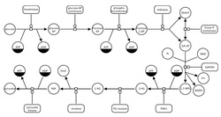
Suppose we take “applied mathematics” in an extremely broad sense that includes math developed for use in electrical engineering, population biology, epidemiology, chemistry, and many other fields. Suppose we look for mathematical structures that repeatedly appear in these diverse contexts — especially structures that aren’t familiar to pure mathematicians. What do we find? The answers may give us some clues about how to improve the foundations of mathematics!
This is what I’m talking about at the Category-Theoretic Foundations of Mathematics Workshop at U.C. Irvine this weekend.
You can see my talk slides here. You can click on any picture or anything written in blue in these slides to get more information — for example, references.
This is what I’m talking about at the Category-Theoretic Foundations of Mathematics Workshop at U.C. Irvine this weekend.
You can see my talk slides here. You can click on any picture or anything written in blue in these slides to get more information — for example, references.
